Λ-Type Three-Level: Weak Pulse, With Coupling
Define and Solve
[1]:
mb_solve_json = """
{
  "atom": {
    "fields": [
      {
        "coupled_levels": [[0, 1]],
        "detuning": 0.0,
        "detuning_positive": true,
        "label": "probe",
        "rabi_freq": 1.0e-3,
        "rabi_freq_t_args":
          {
             "ampl": 1.0,
             "centre": 0.0,
             "fwhm": 1.0
          },
        "rabi_freq_t_func": "gaussian"
      },
      {
        "coupled_levels": [[1, 2]],
        "detuning": 0.0,
        "detuning_positive": false,
        "label": "coupling",
        "rabi_freq": 5.0,
        "rabi_freq_t_args":
        {
          "ampl": 1.0,
          "fwhm": 0.2,
          "on": -1.0,
          "off": 9.0
          },
        "rabi_freq_t_func": "ramp_onoff"
      }
    ],
    "num_states": 3
  },
  "t_min": -2.0,
  "t_max": 10.0,
  "t_steps": 120,
  "z_min": -0.2,
  "z_max": 1.2,
  "z_steps": 100,
  "z_steps_inner": 2,
  "interaction_strengths": [10.0, 10.0],
  "savefile": "mbs-lambda-weak-pulse-more-atoms-no-coupling"
}
"""
[2]:
from maxwellbloch import mb_solve
mbs = mb_solve.MBSolve().from_json_str(mb_solve_json)
[3]:
%time Omegas_zt, states_zt = mbs.mbsolve(recalc=False)
Loaded tuple object.
CPU times: user 0 ns, sys: 3.72 ms, total: 3.72 ms
Wall time: 3.73 ms
## Field Output
[4]:
import matplotlib.pyplot as plt
%matplotlib inline
import seaborn as sns
import numpy as np
sns.set_style('darkgrid')

fig = plt.figure(1, figsize=(16, 6))
ax = fig.add_subplot(111)
cmap_range = np.linspace(0.0, 1.0e-3, 11)
cf = ax.contourf(mbs.tlist, mbs.zlist,
                 np.abs(mbs.Omegas_zt[0]/(2*np.pi)),
                 cmap_range, cmap=plt.cm.Blues)
ax.set_title('Rabi Frequency ($\Gamma / 2\pi $)')
ax.set_xlabel('Time ($1/\Gamma$)')
ax.set_ylabel('Distance ($L$)')
for y in [0.0, 1.0]:
    ax.axhline(y, c='grey', lw=1.0, ls='dotted')
plt.colorbar(cf);

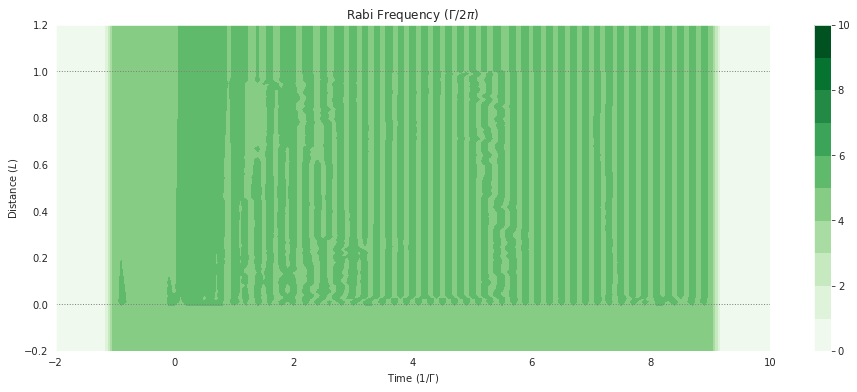
[5]:
import matplotlib.pyplot as plt
%matplotlib inline
import seaborn as sns
import numpy as np
sns.set_style('darkgrid')

fig = plt.figure(1, figsize=(16, 6))
ax = fig.add_subplot(111)
cmap_range = np.linspace(0.0, 10.0, 11)
cf = ax.contourf(mbs.tlist, mbs.zlist,
                 np.abs(mbs.Omegas_zt[1]/(2*np.pi)),
                 cmap_range, cmap=plt.cm.Greens)
ax.set_title('Rabi Frequency ($\Gamma / 2\pi $)')
ax.set_xlabel('Time ($1/\Gamma$)')
ax.set_ylabel('Distance ($L$)')
for y in [0.0, 1.0]:
    ax.axhline(y, c='grey', lw=1.0, ls='dotted')
plt.colorbar(cf);
## Analysis
With no coupling, the weak probe pulse is absorbed just like in the two-level atom case.