Two-Level: Sech Pulse 4π — Pulse Breakup

Define the Problem

First we need to define a sech pulse with the area we want. We’ll fix the width of the pulse and the area to find the right amplitude.

The full-width at half maximum (FWHM) \(t_s\) of the sech pulse is related to the FWHM of a Gaussian by a factor of \(1/2.6339157938\). (See §3.2.2 of my PhD thesis).

import numpy as np

SECH_FWHM_CONV = 1./2.6339157938
t_width = 1.0*SECH_FWHM_CONV # [τ]
print('t_width', t_width)

t_width 0.3796628587572578

mb_solve_json = """
{
  "atom": {
    "fields": [
      {
        "coupled_levels": [[0, 1]],
        "rabi_freq_t_args": {
          "n_pi": 4.0,
          "centre": 0.0,
          "width": %f
        },
        "rabi_freq_t_func": "sech"
      }
    ],
    "num_states": 2
  },
  "t_min": -2.0,
  "t_max": 10.0,
  "t_steps": 240,
  "z_min": -0.5,
  "z_max": 1.5,
  "z_steps": 100,
  "interaction_strengths": [
    10.0
  ],
  "savefile": "mbs-two-sech-4pi"
}
"""%(t_width)

from maxwellbloch import mb_solve
mbs = mb_solve.MBSolve().from_json_str(mb_solve_json)

We’ll just check that the pulse area is what we want.

print('The input pulse area is {0}'.format(
    np.trapz(mbs.Omegas_zt[0,0,:].real, mbs.tlist)/np.pi))

The input pulse area is 3.986854595865458

Omegas_zt, states_zt = mbs.mbsolve(recalc=False)

Loaded tuple object.

Plot Output

import matplotlib.pyplot as plt
%matplotlib inline
import seaborn as sns

sns.set_style('darkgrid')
fig = plt.figure(1, figsize=(16, 6))
ax = fig.add_subplot(111)
cmap_range = np.linspace(0.0, 3.0, 11)
cf = ax.contourf(mbs.tlist, mbs.zlist,
                 np.abs(mbs.Omegas_zt[0]/(2*np.pi)),
                 cmap_range, cmap=plt.cm.Blues)
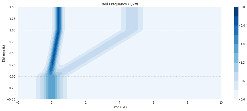
ax.set_title('Rabi Frequency ($\Gamma / 2\pi $)')
ax.set_xlabel('Time ($1/\Gamma$)')
ax.set_ylabel('Distance ($L$)')
for y in [0.0, 1.0]:
    ax.axhline(y, c='grey', lw=1.0, ls='dotted')
plt.colorbar(cf);

fig, ax = plt.subplots(figsize=(16, 5))
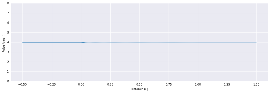
ax.plot(mbs.zlist, mbs.fields_area()[0]/np.pi)
ax.set_ylim([0.0, 8.0])
ax.set_xlabel('Distance ($L$)')
ax.set_ylabel('Pulse Area ($\pi$)')

Text(0, 0.5, 'Pulse Area ($\\pi$)')

Analysis

The \(4 \pi\) sech pulse breaks up into two \(2 \pi\) pulses, which travel at a speed according to their width.

Movie

# C = 0.1 # speed of light
# Y_MIN = 0.0 # Y-axis min
# Y_MAX = 4.0 # y-axis max
# ZOOM = 2 # level of linear interpolation
# FPS = 60 # frames per second
# ATOMS_ALPHA = 0.2 # Atom indicator transparency

# FNAME = "images/mb-solve-two-sech-4pi"
# FNAME_JSON = FNAME + '.json'
# with open(FNAME_JSON, "w") as f:
#     f.write(mb_solve_json)

# !make-mp4-fixed-frame.py -f $FNAME_JSON -c $C --fps $FPS --y-min $Y_MIN --y-max $Y_MAX \
#     --zoom $ZOOM --atoms-alpha $ATOMS_ALPHA #--peak-line --c-line

# FNAME_MP4 = FNAME + '.mp4'
# !make-gif-ffmpeg.sh -f $FNAME_MP4 --in-fps $FPS

# from IPython.display import Image
# Image(url=FNAME_MP4 +'.gif', format='gif')