Two-Level: Weak Square Pulse with Decay

## Define and Solve

mb_solve_json = """
{
  "atom": {
    "decays": [
      {
        "channels": [[0, 1]],
        "rate": 1.0
      }
    ],
    "energies": [],
    "fields": [
      {
        "coupled_levels": [[0, 1]],
        "detuning": 0.0,
        "rabi_freq": 1.0e-3,
        "rabi_freq_t_args": {
          "ampl": 1.0,
          "on": -0.5,
          "off": 0.5
        },
        "rabi_freq_t_func": "square"
      }
    ],
    "num_states": 2
  },
  "t_min": -2.0,
  "t_max": 10.0,
  "t_steps": 100,
  "z_min": -0.2,
  "z_max": 1.2,
  "z_steps": 20,
  "interaction_strengths": [
    1.0
  ]
}
"""

from maxwellbloch import mb_solve
mbs = mb_solve.MBSolve().from_json_str(mb_solve_json)

Omegas_zt, states_zt = mbs.mbsolve()

10.0%. Run time:   0.14s. Est. time left: 00:00:00:01
20.0%. Run time:   0.43s. Est. time left: 00:00:00:01
30.0%. Run time:   0.76s. Est. time left: 00:00:00:01
40.0%. Run time:   1.06s. Est. time left: 00:00:00:01
50.0%. Run time:   1.36s. Est. time left: 00:00:00:01
60.0%. Run time:   1.66s. Est. time left: 00:00:00:01
70.0%. Run time:   1.99s. Est. time left: 00:00:00:00
80.0%. Run time:   2.32s. Est. time left: 00:00:00:00
90.0%. Run time:   2.65s. Est. time left: 00:00:00:00
Total run time:   3.00s

import matplotlib.pyplot as plt
%matplotlib inline
import seaborn as sns
import numpy as np
sns.set_style('darkgrid')

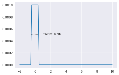
Check the Input Pulse Profile

We’ll just confirm that the input pulse has the profile that we want: a Gaussian with an amplitude of \(1.0 \Gamma\) and a full-width at half maximum (FWHM) of \(1.0 \tau\).

from scipy import interpolate

plt.plot(mbs.tlist, Omegas_zt[0,0].real/(2*np.pi))

half_max = np.max(Omegas_zt[0,0].real/(2*np.pi))/2
spline = interpolate.UnivariateSpline(mbs.tlist,
                                      (Omegas_zt[0,0].real/(2*np.pi)-half_max), s=0)
r1, r2 = spline.roots()

# draw line at FWHM
plt.hlines(y=half_max, xmin=r1, xmax=r2, linestyle='dotted')
plt.annotate('FWHM: ' + '%0.2f'%(r2 - r1), xy=((r2+r1)/2, half_max),
              xycoords='data',
              xytext=(25, 0), textcoords='offset points');

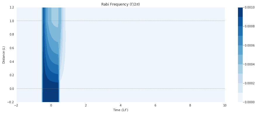
Field Output

fig = plt.figure(1, figsize=(16, 6))
ax = fig.add_subplot(111)
cmap_range = np.linspace(0.0, 1.0e-3, 11)
cf = ax.contourf(mbs.tlist, mbs.zlist,
                 np.abs(mbs.Omegas_zt[0]/(2*np.pi)),
                 cmap_range, cmap=plt.cm.Blues)
ax.set_title('Rabi Frequency ($\Gamma / 2\pi $)')
ax.set_xlabel('Time ($1/\Gamma$)')
ax.set_ylabel('Distance ($L$)')
for y in [0.0, 1.0]:
    ax.axhline(y, c='grey', lw=1.0, ls='dotted')
plt.colorbar(cf);