Velocity Classes for Modelling Doppler Broadening in Thermal Systems
So far the models we have considered are appropriate for ultracold systems with close-to-stationary atoms. For thermal atoms we might want to consider the averaging effect of motion in the line of propagation.
An atom moving with a velocity component \(v\) in the \(z\)-direction will interact with a Doppler-shifted field frequency \(\omega - kv\). This shift is effected over a 1D Maxwell-Boltzmann probability distribution function of velocity
where the thermal width \(u = kv_w\), \(k\) is the wavenumber of the monochromatic field and \(v_w = 2k_b T/ M\) is the most probable speed of the Maxwell-Boltzmann distribution for a temperature \(T\) and atomic mass \(m\).
In MaxwellBloch we model this by solving the system over a range of velocity_classes, each detuning the system from resonance. The results are convoluted over the Maxwell-Boltzmann distribution. The thermal width is provided in thermal_width in the same \(2\pi~\Gamma\) units as the decays and rabi_freqs. We provide velocity classes from thermal_delta_min to thermal_delta_max, again in units of \(2\pi~\Gamma\). The number of classes we choose to solve is given
in thermal_delta_steps.
[1]:
# Imports for plotting
import matplotlib.pyplot as plt

%matplotlib inline
import numpy as np
import seaborn as sns

sns.set_style("darkgrid")
[2]:
mb_solve_json = """
{
  "atom": {
    "decays": [
      {
        "channels": [[0, 1]],
        "rate": 1.0
      }
    ],
    "fields": [
      {
        "coupled_levels": [[0, 1]],
        "rabi_freq": 1.0e-3,
        "rabi_freq_t_args": {
          "ampl": 1.0,
          "centre": 0.0,
          "fwhm": 1.0
        },
        "rabi_freq_t_func": "gaussian"
      }
    ],
    "num_states": 2
  },
  "t_min": -2.0,
  "t_max": 10.0,
  "t_steps": 1000,
  "z_min": -0.2,
  "z_max": 1.2,
  "z_steps": 50,
  "interaction_strengths": [
    1.0
  ],
  "velocity_classes": {
    "thermal_delta_min": -0.1,
    "thermal_delta_max": 0.1,
    "thermal_delta_steps": 4,
    "thermal_width": 0.05
  },
  "savefile": "velocity-classes"
}
"""
[3]:
from maxwellbloch import mb_solve

mbs = mb_solve.MBSolve().from_json_str(mb_solve_json)
We can check the set of velocity classes we’ve defined:
[4]:
mbs.thermal_delta_list / (2 * np.pi)
[4]:
array([-0.1 , -0.05, 0. , 0.05, 0.1 ])
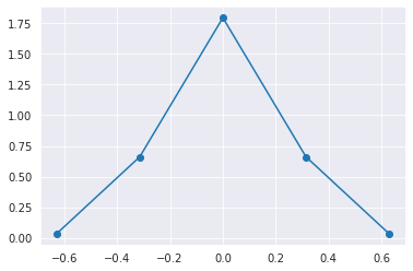
The weights of the Maxwell-Boltzmann distribution at these deltas is given by:
[5]:
mbs.thermal_weights
[5]:
array([0.03289253, 0.6606641 , 1.79587122, 0.6606641 , 0.03289253])
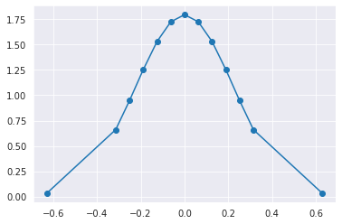
And so we can plot the numerical approximation to the Gaussian Maxwell-Boltzmann distribution:
[6]:
maxboltz = mb_solve.maxwell_boltzmann(
    mbs.thermal_delta_list, 2 * np.pi * mbs.velocity_classes["thermal_width"]
)
plt.plot(mbs.thermal_delta_list, maxboltz, marker="o");
It is useful to look at what the numerical integration looks like for these velocity classes. If it is close to 1, the thermal distribution should be well covered.
[7]:
np.trapezoid(mbs.thermal_weights, mbs.thermal_delta_list)
[7]:
np.float64(0.9896305736453971)
Now we can solve as before. Now at each \(z\)-step, the system will be solved thermal_delta_steps times, once for each velocity class, and so the time taken to solve scales linearly.
[8]:
Omegas_zt, states_zt = mbs.mbsolve(recalc=False)
/home/docs/checkouts/readthedocs.org/user_builds/maxwellbloch/envs/stable/lib/python3.11/site-packages/maxwellbloch/mb_solve.py:344: UserWarning: Savefile was built with maxwellbloch==0.10.0, current version is 0.12.0.
  self.load_results()
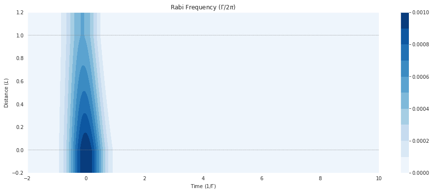
Results in the Time Domain
[9]:
fig = plt.figure(1, figsize=(16, 6))
ax = fig.add_subplot(111)
cmap_range = np.linspace(0.0, 1.0e-3, 11)
cf = ax.contourf(
    mbs.tlist,
    mbs.zlist,
    np.abs(mbs.Omegas_zt[0] / (2 * np.pi)),
    cmap_range,
    cmap=plt.cm.Blues,
)
ax.set_title(r"Rabi Frequency ($\Gamma / 2\pi $)")
ax.set_xlabel(r"Time ($1/\Gamma$)")
ax.set_ylabel("Distance ($L$)")
for y in [0.0, 1.0]:
    ax.axhline(y, c="grey", lw=1.0, ls="dotted")
plt.colorbar(cf);
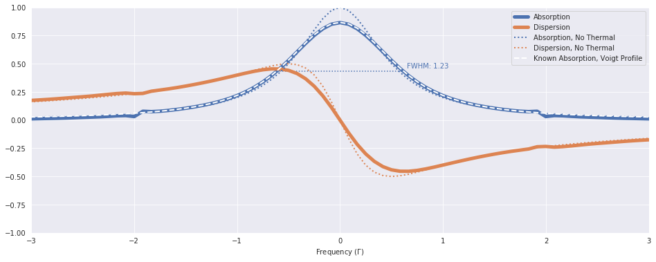
Results in the Frequency Domain
For a two-level system in the linear regime, this convolution of a Lorentzian function with a Gaussian can be determined analytically and is known as a Voigt profile. It is provided in MaxwellBloch as spectral.voigt_two_linear_known(freq_list, decay_rate, thermal_width) so we can compare the simulation solution with the known analytic result.
[10]:
from maxwellbloch import spectral, utility
[11]:
interaction_strength = mbs.interaction_strengths[0]
decay_rate = mbs.atom.decays[0]["rate"]
freq_list = spectral.freq_list(mbs)
absorption_linear_known = spectral.absorption_two_linear_known(
    freq_list, interaction_strength, decay_rate
)
dispersion_linear_known = spectral.dispersion_two_linear_known(
    freq_list, interaction_strength, decay_rate
)

fig = plt.figure(4, figsize=(16, 6))
ax = fig.add_subplot(111)
pal = sns.color_palette("deep")

ax.plot(
    freq_list, spectral.absorption(mbs, 0, -1), label="Absorption", lw=5.0, c=pal[0]
)
ax.plot(
    freq_list, spectral.dispersion(mbs, 0, -1), label="Dispersion", lw=5.0, c=pal[1]
)

ax.plot(
    freq_list,
    absorption_linear_known,
    ls="dotted",
    c=pal[0],
    lw=2.0,
    label="Absorption, No Thermal",
)
ax.plot(
    freq_list,
    dispersion_linear_known,
    ls="dotted",
    c=pal[1],
    lw=2.0,
    label="Dispersion, No Thermal",
)

# Widths
hm, r1, r2 = utility.half_max_roots(freq_list, spectral.absorption(mbs, field_idx=0))
plt.hlines(y=hm, xmin=r1, xmax=r2, linestyle="dotted", color=pal[0])
plt.annotate(
    "FWHM: " + "%0.2f" % (r2 - r1),
    xy=(r2, hm),
    color=pal[0],
    xycoords="data",
    xytext=(5, 5),
    textcoords="offset points",
)

voigt = spectral.voigt_two_linear_known(freq_list, 1.0, 0.05).imag
ax.plot(
    freq_list,
    voigt,
    c="white",
    ls="dashed",
    lw=2.0,
    label="Known Absorption, Voigt Profile",
)

ax.set_xlim(-3.0, 3.0)
ax.set_ylim(-1.0, 1.0)
ax.set_xlabel(r"Frequency ($\Gamma$)")

ax.legend();
[12]:
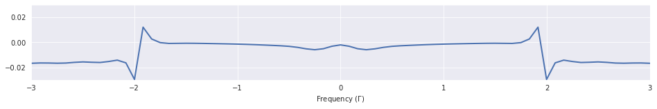
# Plot residuals
fig = plt.figure(figsize=(16, 2))
ax = fig.add_subplot(111)
ax.plot(
    freq_list,
    spectral.absorption(mbs, 0, -1) - voigt,
    label="Absorption",
    lw=2.0,
    c=pal[0],
)
ax.set_xlim(-3.0, 3.0)
ax.set_ylim(-3e-2, 3e-2)
ax.set_xlabel(r"Frequency ($\Gamma$)");
Adding Inner Steps
If the thermal width is much larger than the decay rate, you may wish to add a narrower band around the resonance frequency to sample the Lorentzian sufficiently while covering the Maxwell-Boltzmann distribution efficiently. This can be done by providing an inner range defined by thermal_delta_inner_min, thermal_delta_inner_min and thermal_delta_inner_steps. Any duplicated velocity classes (in the constructed thermal_delta_list) will only be counted once. Below is an example.
[13]:
vc = {
    "thermal_delta_min": -0.1,
    "thermal_delta_max": 0.1,
    "thermal_delta_steps": 4,
    "thermal_delta_inner_min": -0.05,
    "thermal_delta_inner_max": 0.05,
    "thermal_delta_inner_steps": 10,
    "thermal_width": 0.05,
}
So the thermal delta range is \([-0.1, -0.05, 0.05, 1.0]\) and the inner range is \([-0.05, -0.04, \dots, 0.04, 0.05]\). These are combined to form:
[14]:
mbs.build_velocity_classes(velocity_classes=vc)
print(mbs.thermal_delta_list / (2 * np.pi))
[-0.1  -0.05 -0.04 -0.03 -0.02 -0.01  0.    0.01  0.02  0.03  0.04  0.05
  0.1 ]
[15]:
maxboltz = mb_solve.maxwell_boltzmann(
    mbs.thermal_delta_list, 2 * np.pi * mbs.velocity_classes["thermal_width"]
)
plt.plot(mbs.thermal_delta_list, maxboltz, marker="o");