Ladder-Type Three-Level: Weak Pulse with Coupling — EIT
Define the Problem
[1]:
mb_solve_json = """
{
  "atom": {
    "decays": [
      { "channels": [[0,1]],
        "rate": 1.0
      },
      { "channels": [[1,2]],
        "rate": 1.0e-3
      }
    ],
    "fields": [
      {
        "coupled_levels": [[0, 1]],
        "detuning": 5.0,
        "detuning_positive": true,
        "label": "probe",
        "rabi_freq": 1.0e-3,
        "rabi_freq_t_args":
          {
             "ampl": 1.0,
             "centre": 0.0,
             "fwhm": 1.0
          },
        "rabi_freq_t_func": "gaussian"
      },
      {
        "coupled_levels": [[1, 2]],
        "detuning": 0.0,
        "detuning_positive": true,
        "label": "coupling",
        "rabi_freq": 5.0,
        "rabi_freq_t_args":
        {
          "ampl": 1.0,
          "fwhm": 0.2,
          "on": -1.0,
          "off": 9.0
          },
        "rabi_freq_t_func": "ramp_onoff"
      }
    ],
    "num_states": 3
  },
  "t_min": -2.0,
  "t_max": 10.0,
  "t_steps": 60,
  "z_min": -0.2,
  "z_max": 1.2,
  "z_steps": 100,
  "z_steps_inner": 2,
  "interaction_strengths": [100.0, 100.0],
  "savefile": "mbs-ladder-weak-pulse-coupling-decay"
}
"""
[2]:
from maxwellbloch import mb_solve

mb_solve_00 = mb_solve.MBSolve().from_json_str(mb_solve_json)
## Solve the Problem
[3]:
%time Omegas_zt, states_zt = mb_solve_00.mbsolve(recalc=False)
CPU times: user 542 μs, sys: 1.11 ms, total: 1.66 ms
Wall time: 1.85 ms
/home/docs/checkouts/readthedocs.org/user_builds/maxwellbloch/envs/v0.10.0/lib/python3.11/site-packages/qutip/fileio.py:253: VisibleDeprecationWarning: dtype(): align should be passed as Python or NumPy boolean but got `align=0`. Did you mean to pass a tuple to create a subarray type? (Deprecated NumPy 2.4)
  out = pickle.load(fileObject, encoding='latin1')
/home/docs/checkouts/readthedocs.org/user_builds/maxwellbloch/envs/v0.10.0/lib/python3.11/site-packages/maxwellbloch/mb_solve.py:324: UserWarning: Savefile mbs-ladder-weak-pulse-coupling-decay.qu has no integrity metadata (old format). Loading without hash check.
  self.load_results()
## Plot Output
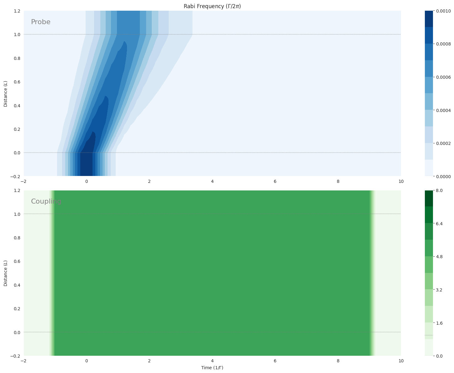
[4]:
import matplotlib.pyplot as plt

%matplotlib inline
import seaborn as sns

sns.set_style("dark")

import numpy as np

fig = plt.figure(1, figsize=(16, 12))

# Probe
ax = fig.add_subplot(211)
cmap_range = np.linspace(0.0, 1.0e-3, 11)
cf = ax.contourf(
    mb_solve_00.tlist,
    mb_solve_00.zlist,
    np.abs(mb_solve_00.Omegas_zt[0] / (2 * np.pi)),
    cmap_range,
    cmap=plt.cm.Blues,
)
ax.set_title(r"Rabi Frequency ($\Gamma / 2\pi $)")
ax.set_ylabel("Distance ($L$)")
ax.text(
    0.02,
    0.95,
    "Probe",
    verticalalignment="top",
    horizontalalignment="left",
    transform=ax.transAxes,
    color="grey",
    fontsize=16,
)
plt.colorbar(cf)

# Coupling
ax = fig.add_subplot(212)
cmap_range = np.linspace(0.0, 8.0, 11)
cf = ax.contourf(
    mb_solve_00.tlist,
    mb_solve_00.zlist,
    np.abs(mb_solve_00.Omegas_zt[1] / (2 * np.pi)),
    cmap_range,
    cmap=plt.cm.Greens,
)
ax.set_xlabel(r"Time ($1/\Gamma$)")
ax.set_ylabel("Distance ($L$)")
ax.text(
    0.02,
    0.95,
    "Coupling",
    verticalalignment="top",
    horizontalalignment="left",
    transform=ax.transAxes,
    color="grey",
    fontsize=16,
)
plt.colorbar(cf)

# Both
for ax in fig.axes:
    for y in [0.0, 1.0]:
        ax.axhline(y, c="grey", lw=1.0, ls="dotted")
plt.tight_layout();