Λ-Type Three-Level: Weak Pulse with Coupling in a Cloud — Pulse Compression

## Define and Solve

mb_solve_json = """
{
  "atom": {
    "fields": [
      {
        "coupled_levels": [[0, 1]],
        "detuning": 0.0,
        "detuning_positive": true,
        "label": "probe",
        "rabi_freq": 1.0e-3,
        "rabi_freq_t_args":
          {
             "ampl": 1.0,
             "centre": 0.0,
             "fwhm": 1.0
          },
        "rabi_freq_t_func": "gaussian"
      },
      {
        "coupled_levels": [[1, 2]],
        "detuning": 0.0,
        "detuning_positive": false,
        "label": "coupling",
        "rabi_freq": 5.0,
        "rabi_freq_t_args":
        {
          "ampl": 1.0,
          "fwhm": 0.2,
          "on": -1.0,
          "off": 9.0
          },
        "rabi_freq_t_func": "ramp_onoff"
      }
    ],
    "num_states": 3
  },
  "t_min": -2.0,
  "t_max": 10.0,
  "t_steps": 120,
  "z_min": -0.2,
  "z_max": 1.2,
  "z_steps": 70,
  "z_steps_inner": 100,
  "num_density_z_func": "gaussian",
  "num_density_z_args": {
    "ampl": 1.0,
    "fwhm": 0.5,
    "centre": 0.5
  },
  "interaction_strengths": [1.0e3, 1.0e3],
  "savefile": "mbs-lambda-weak-pulse-cloud-atoms-some-coupling"
}
"""

from maxwellbloch import mb_solve

mbs = mb_solve.MBSolve().from_json_str(mb_solve_json)

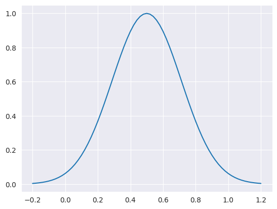
Number Density Profile

In this case we’ve defined a non-square profile for the number density as a function of \(z\) (num_density_z_func).

import matplotlib.pyplot as plt

%matplotlib inline
import seaborn as sns

sns.set_style("darkgrid")

plt.plot(mbs.zlist, mbs.num_density_z_func(mbs.zlist, mbs.num_density_z_args));

%time Omegas_zt, states_zt = mbs.mbsolve(recalc=False)

CPU times: user 964 μs, sys: 995 μs, total: 1.96 ms
Wall time: 5.48 ms

/home/docs/checkouts/readthedocs.org/user_builds/maxwellbloch/envs/v0.10.0/lib/python3.11/site-packages/qutip/fileio.py:253: VisibleDeprecationWarning: dtype(): align should be passed as Python or NumPy boolean but got `align=0`. Did you mean to pass a tuple to create a subarray type? (Deprecated NumPy 2.4)
  out = pickle.load(fileObject, encoding='latin1')
/home/docs/checkouts/readthedocs.org/user_builds/maxwellbloch/envs/v0.10.0/lib/python3.11/site-packages/maxwellbloch/mb_solve.py:324: UserWarning: Savefile mbs-lambda-weak-pulse-cloud-atoms-some-coupling.qu has no integrity metadata (old format). Loading without hash check.
  self.load_results()

## Plot Output

import numpy as np

fig = plt.figure(1, figsize=(16, 12))

# Probe
ax = fig.add_subplot(211)
cmap_range = np.linspace(0.0, 1.0e-3, 11)
cf = ax.contourf(
    mbs.tlist,
    mbs.zlist,
    np.abs(mbs.Omegas_zt[0] / (2 * np.pi)),
    cmap_range,
    cmap=plt.cm.Blues,
)
ax.set_title(r"Rabi Frequency ($\Gamma / 2\pi $)")
ax.set_ylabel("Distance ($L$)")
ax.text(
    0.02,
    0.95,
    "Probe",
    verticalalignment="top",
    horizontalalignment="left",
    transform=ax.transAxes,
    color="grey",
    fontsize=16,
)
plt.colorbar(cf)

# Coupling
ax = fig.add_subplot(212)
cmap_range = np.linspace(0.0, 8.0, 11)
cf = ax.contourf(
    mbs.tlist,
    mbs.zlist,
    np.abs(mbs.Omegas_zt[1] / (2 * np.pi)),
    cmap_range,
    cmap=plt.cm.Greens,
)
ax.set_xlabel(r"Time ($1/\Gamma$)")
ax.set_ylabel("Distance ($L$)")
ax.text(
    0.02,
    0.95,
    "Coupling",
    verticalalignment="top",
    horizontalalignment="left",
    transform=ax.transAxes,
    color="grey",
    fontsize=16,
)
plt.colorbar(cf)

# Both
for ax in fig.axes:
    for y in [0.0, 1.0]:
        ax.axhline(y, c="grey", lw=1.0, ls="dotted")
plt.tight_layout();

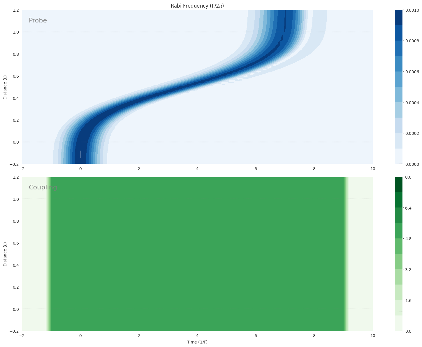
Analysis

From my thesis, §4.3.2.

This high coefficient might correspond to either a particularly long or dense medium. We see from the gradient of the profile that the pulse slows down considerably as the density increases, and speeds up again as it leaves the medium. The overall slow-light effect is large, with the pulse arriving \(8 \tau\) later than it would covering the same distance in vacuo.

At the same time as it is slowed, the spatial extent of the pulse is significantly decreased as it moves into the high-density region. This happens because as the pulse moves into the medium its leading edge slows down before the trailing edge while the field strength remains the same, causing the pulse to ‘bunch up‘. The pulse is compressed by a factor \(v g/c\). In the BEC experiment mentioned above, light pulses were compressed from kilometre to sub-millimetre scale.