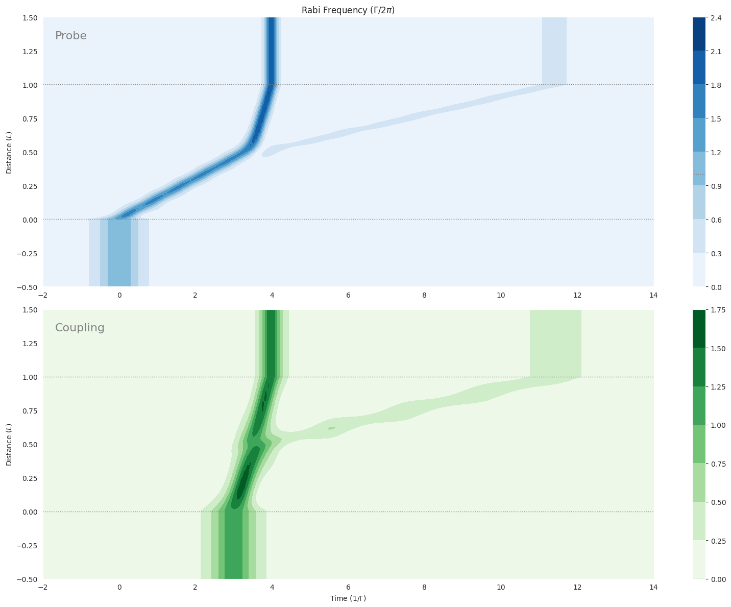
V-Type Three-Level: Solitons form Simulton
In this example, a soliton is put in on both the probe and the coupling fields.
[1]:
import numpy as np

sech_fwhm_conv = 1.0 / 2.6339157938
t_width = 1.0 * sech_fwhm_conv  # [τ]

print("t_width", t_width)

n_1 = np.sqrt(8)  # For a pulse area of nπ
ampl_1 = n_1 / t_width / (2 * np.pi)  # Pulse amplitude [2π Γ]

print("ampl_1", ampl_1)

n_2 = np.sqrt(8)  # For a pulse area of nπ
ampl_2 = n_2 / t_width / (2 * np.pi)  # Pulse amplitude [2π Γ]

print("ampl_2", ampl_2)
t_width 0.3796628587572578
ampl_1 1.1856786822710181
ampl_2 1.1856786822710181
[2]:
np.sqrt(n_1**2 + n_2**2)
[2]:
np.float64(4.0)
[3]:
mb_solve_json = """
{{
  "atom": {{
    "fields": [
      {{
        "coupled_levels": [[0, 1]],
        "label": "probe",
        "rabi_freq": 1.0,
        "rabi_freq_t_args":
          {{
             "ampl": {ampl_1},
             "centre": 0.0,
             "width": {t_width}
          }},
        "rabi_freq_t_func": "sech"
      }},
      {{
        "coupled_levels": [[0, 2]],
        "label": "coupling",
        "rabi_freq": 1.0,
        "rabi_freq_t_args":
          {{
             "ampl": {ampl_2},
             "centre": 3.0,
             "width": {t_width}
          }},
        "rabi_freq_t_func": "sech"
      }}
    ],
    "num_states": 3
  }},
  "t_min": -2.0,
  "t_max": 14.0,
  "t_steps": 200,
  "z_min": -0.5,
  "z_max": 1.5,
  "z_steps": 500,
  "z_steps_inner": 1,
  "interaction_strengths": [50.0, 10.0],
  "savefile": "mbs-vee-sech-sqrt8pi-sqrt8pi-collision"
}}
""".format(ampl_1=ampl_1, t_width=t_width, ampl_2=ampl_2)
[4]:
from maxwellbloch import mb_solve

mb_solve_00 = mb_solve.MBSolve().from_json_str(mb_solve_json)

%time Omegas_zt, states_zt = mb_solve_00.mbsolve(recalc=False, pbar_chunk_size=2)
CPU times: user 51 μs, sys: 8.97 ms, total: 9.02 ms
Wall time: 8.85 ms
/home/docs/checkouts/readthedocs.org/user_builds/maxwellbloch/envs/v0.10.0/lib/python3.11/site-packages/qutip/fileio.py:253: VisibleDeprecationWarning: dtype(): align should be passed as Python or NumPy boolean but got `align=0`. Did you mean to pass a tuple to create a subarray type? (Deprecated NumPy 2.4)
  out = pickle.load(fileObject, encoding='latin1')
/home/docs/checkouts/readthedocs.org/user_builds/maxwellbloch/envs/v0.10.0/lib/python3.11/site-packages/maxwellbloch/mb_solve.py:324: UserWarning: Savefile mbs-vee-sech-sqrt8pi-sqrt8pi-collision.qu has no integrity metadata (old format). Loading without hash check.
  self.load_results()
[5]:
import matplotlib.pyplot as plt

%matplotlib inline
import seaborn as sns

sns.set_style("darkgrid")
fig = plt.figure(1, figsize=(16, 12))

# Probe
ax = fig.add_subplot(211)
# cmap_range = np.linspace(0.0, 0.8, 11)
cf = ax.contourf(
    mb_solve_00.tlist,
    mb_solve_00.zlist,
    np.abs(mb_solve_00.Omegas_zt[0] / (2 * np.pi)),
    #                  cmap_range,
    cmap=plt.cm.Blues,
)
ax.set_title(r"Rabi Frequency ($\Gamma / 2\pi $)")
ax.set_ylabel("Distance ($L$)")
ax.text(
    0.02,
    0.95,
    "Probe",
    verticalalignment="top",
    horizontalalignment="left",
    transform=ax.transAxes,
    color="grey",
    fontsize=16,
)
plt.colorbar(cf)

# Coupling
ax = fig.add_subplot(212)
# cmap_range = np.linspace(0.0, 0.8, 11)
cf = ax.contourf(
    mb_solve_00.tlist,
    mb_solve_00.zlist,
    np.abs(mb_solve_00.Omegas_zt[1] / (2 * np.pi)),
    #                  cmap_range,
    cmap=plt.cm.Greens,
)
ax.set_xlabel(r"Time ($1/\Gamma$)")
ax.set_ylabel("Distance ($L$)")
ax.text(
    0.02,
    0.95,
    "Coupling",
    verticalalignment="top",
    horizontalalignment="left",
    transform=ax.transAxes,
    color="grey",
    fontsize=16,
)
plt.colorbar(cf)

# Both
for ax in fig.axes:
    for y in [0.0, 1.0]:
        ax.axhline(y, c="grey", lw=1.0, ls="dotted")
plt.tight_layout();
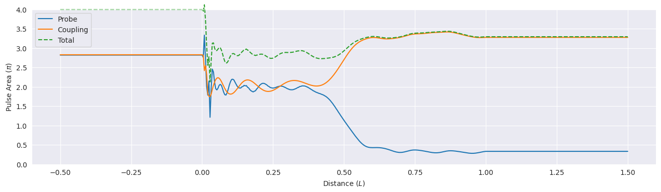
[6]:
total_area = np.sqrt(
    mb_solve_00.fields_area()[0] ** 2 + mb_solve_00.fields_area()[1] ** 2
)

fig, ax = plt.subplots(figsize=(16, 4))
ax.plot(
    mb_solve_00.zlist,
    mb_solve_00.fields_area()[0] / np.pi,
    label="Probe",
    clip_on=False,
)
ax.plot(
    mb_solve_00.zlist,
    mb_solve_00.fields_area()[1] / np.pi,
    label="Coupling",
    clip_on=False,
)
ax.plot(
    mb_solve_00.zlist, total_area / np.pi, label="Total", ls="dashed", clip_on=False
)
ax.legend()
ax.set_ylim([0.0, 4.0])
ax.set_xlabel("Distance ($L$)")
ax.set_ylabel(r"Pulse Area ($\pi$)");
[7]:
fields_area_abs = np.trapezoid(np.abs(mb_solve_00.Omegas_zt), mb_solve_00.tlist, axis=2)
Animation
[8]:
C = 0.1  # speed of light
Y_MIN = 0.0  # Y-axis min
Y_MAX = 3.0  # y-axis max
ZOOM = 2  # level of linear interpolation
FPS = 60  # frames per second
ATOMS_ALPHA = 0.2  # Atom indicator transparency
[9]:
FNAME = "mbs-vee-sech-sqrt8pi-sqrt8pi-collision"
FNAME_JSON = FNAME + ".json"
with open(FNAME_JSON, "w") as f:
    f.write(mb_solve_json)