Λ-Type Three-Level: Weak Pulse, No Coupling

Define and Solve

mb_solve_json = """
{
  "atom": {
    "fields": [
      {
        "coupled_levels": [[0, 1]],
        "detuning": 0.0,
        "detuning_positive": true,
        "label": "probe",
        "rabi_freq": 1.0e-3,
        "rabi_freq_t_args":
          {
             "ampl": 1.0,
             "centre": 0.0,
             "fwhm": 1.0
          },
        "rabi_freq_t_func": "gaussian"
      },
      {
        "coupled_levels": [[1, 2]],
        "detuning": 0.0,
        "detuning_positive": false,
        "label": "coupling",
        "rabi_freq": 0.0,
        "rabi_freq_t_args":
        {
          "ampl": 1.0,
          "fwhm": 0.2,
          "on": -1.0,
          "off": 9.0
          },
        "rabi_freq_t_func": "ramp_onoff"
      }
    ],
    "num_states": 3
  },
  "t_min": -2.0,
  "t_max": 10.0,
  "t_steps": 120,
  "z_min": -0.2,
  "z_max": 1.2,
  "z_steps": 100,
  "z_steps_inner": 2,
  "interaction_strengths": [10.0, 10.0],
  "savefile": "mbs-lambda-weak-pulse-more-atoms-no-coupling"
}
"""

from maxwellbloch import mb_solve

mbs = mb_solve.MBSolve().from_json_str(mb_solve_json)

%time Omegas_zt, states_zt = mbs.mbsolve(recalc=False)

/home/docs/checkouts/readthedocs.org/user_builds/maxwellbloch/envs/v0.11.0/lib/python3.11/site-packages/qutip/solver/solver_base.py:598: FutureWarning: e_ops will be keyword only from qutip 5.3 for all solver
  warnings.warn(
100%|██████████| 100/100 [00:01<00:00, 68.40z/s, Ω_max=0.00154]

Saving MBSolve to mbs-lambda-weak-pulse-more-atoms-no-coupling.qu
CPU times: user 1.47 s, sys: 90.9 ms, total: 1.56 s
Wall time: 1.49 s

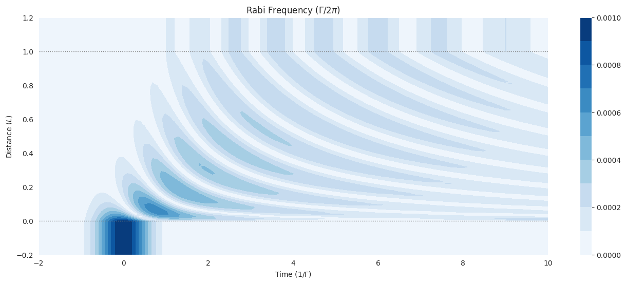
## Field Output

import matplotlib.pyplot as plt

%matplotlib inline
import numpy as np
import seaborn as sns

sns.set_style("darkgrid")

fig = plt.figure(1, figsize=(16, 6))
ax = fig.add_subplot(111)
cmap_range = np.linspace(0.0, 1.0e-3, 11)
cf = ax.contourf(
    mbs.tlist,
    mbs.zlist,
    np.abs(mbs.Omegas_zt[0] / (2 * np.pi)),
    cmap_range,
    cmap=plt.cm.Blues,
)
ax.set_title(r"Rabi Frequency ($\Gamma / 2\pi $)")
ax.set_xlabel(r"Time ($1/\Gamma$)")
ax.set_ylabel("Distance ($L$)")
for y in [0.0, 1.0]:
    ax.axhline(y, c="grey", lw=1.0, ls="dotted")
plt.colorbar(cf);

import matplotlib.pyplot as plt

%matplotlib inline
import numpy as np
import seaborn as sns

sns.set_style("darkgrid")

fig = plt.figure(1, figsize=(16, 6))
ax = fig.add_subplot(111)
cmap_range = np.linspace(0.0, 10.0, 11)
cf = ax.contourf(
    mbs.tlist,
    mbs.zlist,
    np.abs(mbs.Omegas_zt[1] / (2 * np.pi)),
    cmap_range,
    cmap=plt.cm.Greens,
)
ax.set_title(r"Rabi Frequency ($\Gamma / 2\pi $)")
ax.set_xlabel(r"Time ($1/\Gamma$)")
ax.set_ylabel("Distance ($L$)")
for y in [0.0, 1.0]:
    ax.axhline(y, c="grey", lw=1.0, ls="dotted")
plt.colorbar(cf);

## Analysis

With no coupling, the weak probe pulse is absorbed just like in the two-level atom case.