Two-Level: Weak Square Pulse with Decay

## Define and Solve

mb_solve_json = """
{
  "atom": {
    "decays": [
      {
        "channels": [[0, 1]],
        "rate": 1.0
      }
    ],
    "energies": [],
    "fields": [
      {
        "coupled_levels": [[0, 1]],
        "detuning": 0.0,
        "rabi_freq": 1.0e-3,
        "rabi_freq_t_args": {
          "ampl": 1.0,
          "on": -0.5,
          "off": 0.5
        },
        "rabi_freq_t_func": "square"
      }
    ],
    "num_states": 2
  },
  "t_min": -2.0,
  "t_max": 10.0,
  "t_steps": 100,
  "z_min": -0.2,
  "z_max": 1.2,
  "z_steps": 20,
  "interaction_strengths": [
    1.0
  ]
}
"""

from maxwellbloch import mb_solve

mbs = mb_solve.MBSolve().from_json_str(mb_solve_json)

Omegas_zt, states_zt = mbs.mbsolve()

/home/docs/checkouts/readthedocs.org/user_builds/maxwellbloch/envs/v0.11.0/lib/python3.11/site-packages/qutip/solver/solver_base.py:598: FutureWarning: e_ops will be keyword only from qutip 5.3 for all solver
  warnings.warn(
100%|██████████| 20/20 [00:00<00:00, 82.64z/s, Ω_max=0.00534]

import matplotlib.pyplot as plt

%matplotlib inline
import numpy as np
import seaborn as sns

sns.set_style("darkgrid")

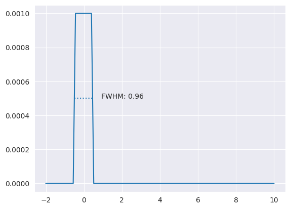
Check the Input Pulse Profile

We’ll just confirm that the input pulse has the profile that we want: a Gaussian with an amplitude of \(1.0 \Gamma\) and a full-width at half maximum (FWHM) of \(1.0 \tau\).

from scipy import interpolate

plt.plot(mbs.tlist, Omegas_zt[0, 0].real / (2 * np.pi))

half_max = np.max(Omegas_zt[0, 0].real / (2 * np.pi)) / 2
spline = interpolate.UnivariateSpline(
    mbs.tlist, (Omegas_zt[0, 0].real / (2 * np.pi) - half_max), s=0
)
r1, r2 = spline.roots()

# draw line at FWHM
plt.hlines(y=half_max, xmin=r1, xmax=r2, linestyle="dotted")
plt.annotate(
    "FWHM: " + "%0.2f" % (r2 - r1),
    xy=((r2 + r1) / 2, half_max),
    xycoords="data",
    xytext=(25, 0),
    textcoords="offset points",
);

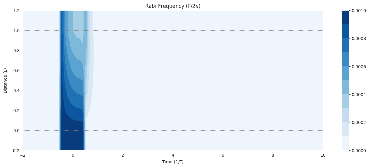
Field Output

fig = plt.figure(1, figsize=(16, 6))
ax = fig.add_subplot(111)
cmap_range = np.linspace(0.0, 1.0e-3, 11)
cf = ax.contourf(
    mbs.tlist,
    mbs.zlist,
    np.abs(mbs.Omegas_zt[0] / (2 * np.pi)),
    cmap_range,
    cmap=plt.cm.Blues,
)
ax.set_title(r"Rabi Frequency ($\Gamma / 2\pi $)")
ax.set_xlabel(r"Time ($1/\Gamma$)")
ax.set_ylabel("Distance ($L$)")
for y in [0.0, 1.0]:
    ax.axhline(y, c="grey", lw=1.0, ls="dotted")
plt.colorbar(cf);