[1]:
# Imports for plotting

import matplotlib.pyplot as plt

%matplotlib inline
import numpy as np
import seaborn as sns

sns.set_style("darkgrid")
Built-in Time Functions
Field profiles are defined as functions of time. A base rabi_freq is multiplied by a time function rabi_freq_t_func and related arguments rabi_freq_t_args. For example, a Gaussian pulse with a peak of \(\Omega_0 = 2\pi \cdot 0.001 \mathrm{~ MHz}\) and a full-width at half-maximum (FWHM) of \(1 \mathrm{~ \mu s}\) arriving at the start of the medium at \(t = 0 \mathrm{~ \mu s}\) can be specified in JSON with "rabi_freq": 1.0e-3, "rabi_freq_t_func": "gaussian", and
"rabi_freq_t_args": {"ampl": 1.0, "centre": 0.0, "fwhm": 1.0}.
Here we’ll show all of the built-in t_funcs you can use. It is also possible to write your own.
[2]:
from maxwellbloch import t_funcs

tlist = np.linspace(0.0, 1.0, 201)
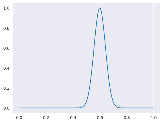
Gaussian
The Gaussian profile is defined as
where \(t_0\) (centre) is the point at which the function reaches its peak amplitude \(\Omega_0\) (ampl). The width \(t_w\) (fwhm) is the full width at half maximum (FWHM) of a Gaussian.
[3]:
plt.plot(
    tlist,
    t_funcs.gaussian(1)(tlist, args={"ampl_1": 1.0, "fwhm_1": 0.1, "centre_1": 0.6}),
);
Note
Why are these args written like ampl_1 here instead of ampl? In the t_funcs module, each built-in time profile is specified in a functor that takes an index as argument and returns a function whose t_args are suffixed with that index. This is because when we have multiple fields, MaxwellBloch needs to be able to distinguish the arguments of each function. When specifying MaxwellBloch problems, you won’t need to worry about this.
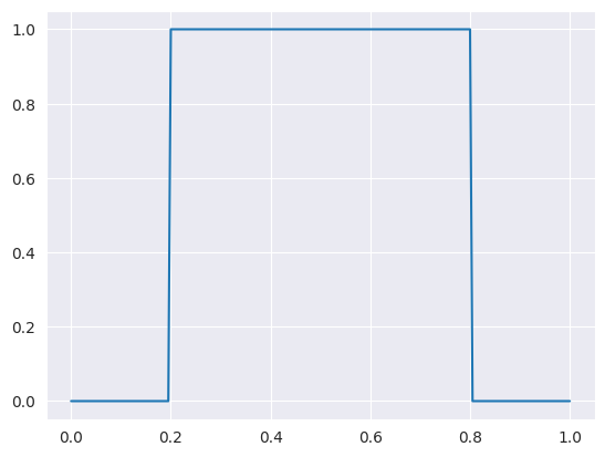
Square
The square profile just needs an amplitude ampl and switch on and off times.
[4]:
plt.plot(
    tlist, t_funcs.square(1)(tlist, args={"ampl_1": 1.0, "on_1": 0.2, "off_1": 0.8})
);
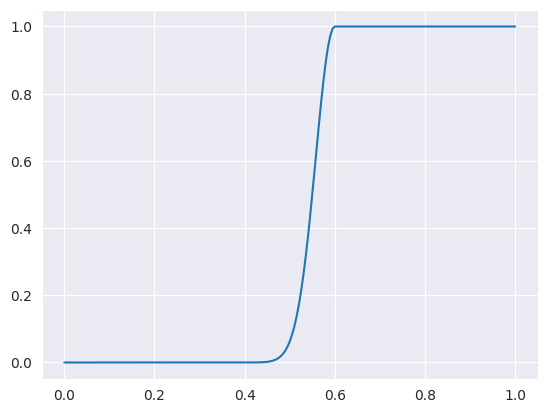
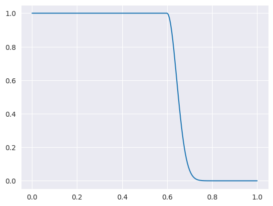
Ramp On
The ramp on and off functions use a Gaussian profile to reach peak amplitude. For example, the ramp_on function is
where \(t_0\) (centre_1) is the point at which the function reaches its peak amplitude \(\Omega_0\) (ampl_1). The duration of the ramp-on is governed by \(t_w\) (fwhm_1), which is the full width at half maximum (FWHM) of a Gaussian. The ramp_off, ramp_onoff and ramp_offon functions behave in the same way.
[5]:
plt.plot(
    tlist, t_funcs.ramp_on(1)(tlist, args={"ampl_1": 1.0, "fwhm_1": 0.1, "on_1": 0.6})
);
Ramp Off
[6]:
plt.plot(
    tlist, t_funcs.ramp_off(1)(tlist, args={"ampl_1": 1.0, "fwhm_1": 0.1, "off_1": 0.6})
);
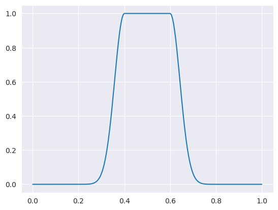
Ramp On and Off
[7]:
plt.plot(
    tlist,
    t_funcs.ramp_onoff(1)(
        tlist, args={"ampl_1": 1.0, "fwhm_1": 0.1, "on_1": 0.4, "off_1": 0.6}
    ),
);
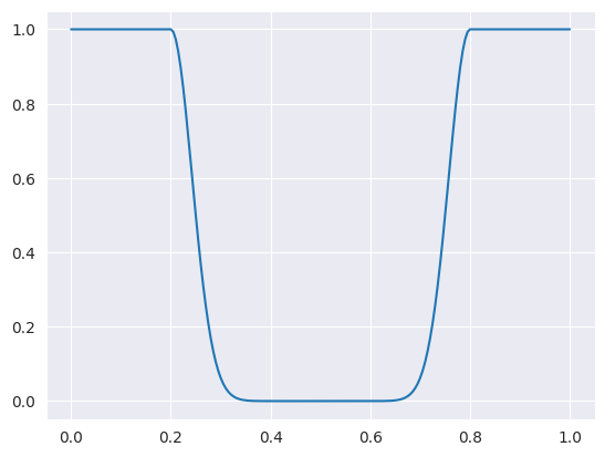
Ramp Off and On
[8]:
plt.plot(
    tlist,
    t_funcs.ramp_offon(1)(
        tlist, args={"ampl_1": 1.0, "fwhm_1": 0.1, "off_1": 0.2, "on_1": 0.8}
    ),
);
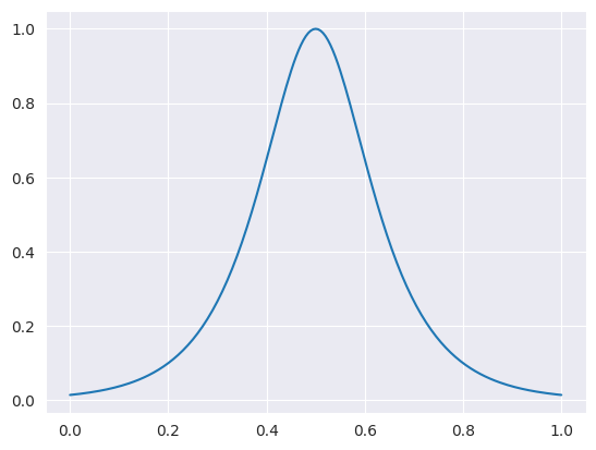
Sech
The hyperbolic secant (sech) function is defined by
where \(t_0\) (centre_1) is the point at which the function reaches its peak amplitude \(\Omega_0\) (ampl_1). The width is governed by \(t_w\) (width_1).
[9]:
plt.plot(
    tlist, t_funcs.sech(1)(tlist, args={"ampl_1": 1.0, "width_1": 0.1, "centre_1": 0.5})
);
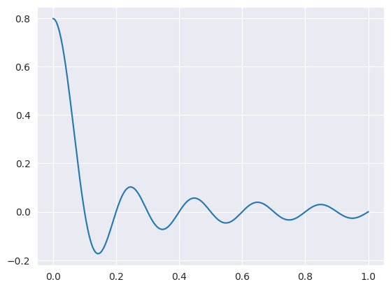
Sinc
The cardinal sine (sinc) function is defined by
where \(w\) is a width function and \(\Omega_0\) (ampl_1) is the peak amplitude of the function.
[10]:
plt.plot(tlist, t_funcs.sinc(1)(tlist, args={"ampl_1": 1.0, "width_1": 10.0}));
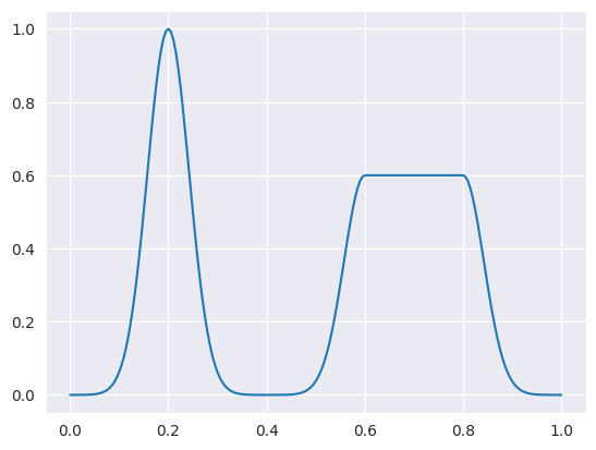
Combining Time Functions
It is possible to create your own time functions, or combine the built-in time functions. To do this you have to pass the function into the Field object directly, it’s not possible to specify in JSON.
[11]:
f = lambda t, args: t_funcs.gaussian(1)(t, args) + t_funcs.ramp_onoff(2)(t, args)
plt.plot(
    tlist,
    f(
        tlist,
        args={
            "ampl_1": 1.0,
            "fwhm_1": 0.1,
            "centre_1": 0.2,
            "ampl_2": 0.6,
            "fwhm_2": 0.1,
            "on_2": 0.6,
            "off_2": 0.8,
        },
    ),
);
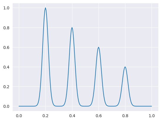
[12]:
g = lambda t, args: (
    t_funcs.gaussian(1)(t, args)
    + t_funcs.gaussian(2)(t, args)
    + t_funcs.gaussian(3)(t, args)
    + t_funcs.gaussian(4)(t, args)
)
plt.plot(
    tlist,
    g(
        tlist,
        args={
            "ampl_1": 1.0,
            "fwhm_1": 0.05,
            "centre_1": 0.2,
            "ampl_2": 0.8,
            "fwhm_2": 0.05,
            "centre_2": 0.4,
            "ampl_3": 0.6,
            "fwhm_3": 0.05,
            "centre_3": 0.6,
            "ampl_4": 0.4,
            "fwhm_4": 0.05,
            "centre_4": 0.8,
        },
    ),
);