Two-Level: Weak CW through More Atoms with Decay

## Define and Solve

mb_solve_json = """
{
  "atom": {
    "decays": [
      {
        "channels": [[0, 1]],
        "rate": 1.0
      }
    ],
    "fields": [
      {
        "coupled_levels": [[0, 1]],
        "detuning": 0.0,
        "rabi_freq": 1.0e-3,
        "rabi_freq_t_args": {
          "ampl": 1.0,
          "on": 0.0,
          "off": 8.0,
          "fwhm": 1.0
        },
        "rabi_freq_t_func": "ramp_onoff"
      }
    ],
    "num_states": 2
  },
  "t_min": -2.0,
  "t_max": 10.0,
  "t_steps": 100,
  "z_min": -0.2,
  "z_max": 1.2,
  "z_steps": 20,
  "interaction_strengths": [
    10.0
  ]
}
"""

from maxwellbloch import mb_solve

mbs = mb_solve.MBSolve().from_json_str(mb_solve_json)

Omegas_zt, states_zt = mbs.mbsolve()

  z-step 2/20 (10%)

/home/docs/checkouts/readthedocs.org/user_builds/maxwellbloch/envs/v0.8.1/lib/python3.11/site-packages/qutip/solver/solver_base.py:598: FutureWarning: e_ops will be keyword only from qutip 5.3 for all solver
  warnings.warn(

  z-step 4/20 (20%)
  z-step 6/20 (30%)
  z-step 8/20 (40%)
  z-step 10/20 (50%)
  z-step 12/20 (60%)
  z-step 14/20 (70%)
  z-step 16/20 (80%)
  z-step 18/20 (90%)

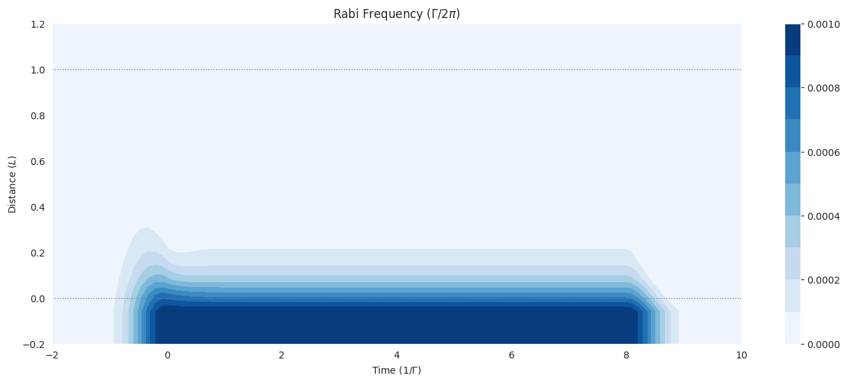
Field Output

import matplotlib.pyplot as plt

%matplotlib inline
import numpy as np
import seaborn as sns

sns.set_style("darkgrid")

fig = plt.figure(1, figsize=(16, 6))
ax = fig.add_subplot(111)
cmap_range = np.linspace(0.0, 1.0e-3, 11)
cf = ax.contourf(
    mbs.tlist,
    mbs.zlist,
    np.abs(mbs.Omegas_zt[0] / (2 * np.pi)),
    cmap_range,
    cmap=plt.cm.Blues,
)
ax.set_title(r"Rabi Frequency ($\Gamma / 2\pi $)")
ax.set_xlabel(r"Time ($1/\Gamma$)")
ax.set_ylabel("Distance ($L$)")
for y in [0.0, 1.0]:
    ax.axhline(y, c="grey", lw=1.0, ls="dotted")
plt.colorbar(cf);