V-Type Three-Level: √8π Sech Pulse, √8π Coupling

import numpy as np

sech_fwhm_conv = 1.0 / 2.6339157938
t_width = 1.0 * sech_fwhm_conv  # [τ]

print(np.sqrt(8))

print("t_width", t_width)

n = np.sqrt(8)  # For a pulse area of nπ
ampl = n / t_width / (2 * np.pi)  # Pulse amplitude [2π Γ]

print("ampl", ampl)

n = np.sqrt(8)  # For a pulse area of nπ
ampl_2 = n / t_width / (2 * np.pi)  # Pulse amplitude [2π Γ]

print("ampl_2", ampl_2)

2.8284271247461903
t_width 0.3796628587572578
ampl 1.1856786822710181
ampl_2 1.1856786822710181

a = np.sqrt(8)
b = np.sqrt(8)

np.sqrt(a**2 + b**2)

np.float64(4.0)

mb_solve_json = """
{
  "atom": {
    "decays": [
      { "channels": [[0,1], [0,2]],
        "rate": 0.0
      }
    ],
    "energies": [],
    "fields": [
      {
        "coupled_levels": [[0, 1]],
        "detuning": 0.0,
        "detuning_positive": true,
        "label": "probe",
        "rabi_freq": 1.18567868227,
        "rabi_freq_t_args":
          {
             "ampl": 1.0,
             "centre": 0.0,
             "width": 0.3796628587572578
          },
        "rabi_freq_t_func": "sech"
      },
      {
        "coupled_levels": [[0, 2]],
        "detuning": 0.0,
        "detuning_positive": true,
        "label": "coupling",
        "rabi_freq": 1.18567868227,
        "rabi_freq_t_args":
          {
             "ampl": 1.0,
             "centre": 0.0,
             "width": 0.3796628587572578
          },
        "rabi_freq_t_func": "sech"
      }
    ],
    "num_states": 3
  },
  "t_min": -2.0,
  "t_max": 10.0,
  "t_steps": 60,
  "z_min": -0.2,
  "z_max": 1.2,
  "z_steps": 70,
  "z_steps_inner": 1,
  "interaction_strengths": [10.0, 10.0],
  "savefile": "mbs-vee-sech-sqrt8pi-sqrt8pi"
}
"""

from maxwellbloch import mb_solve

mb_solve_00 = mb_solve.MBSolve().from_json_str(mb_solve_json)

%time Omegas_zt, states_zt = mb_solve_00.mbsolve(recalc=True)

/home/docs/checkouts/readthedocs.org/user_builds/maxwellbloch/envs/v0.8.1/lib/python3.11/site-packages/qutip/solver/solver_base.py:598: FutureWarning: e_ops will be keyword only from qutip 5.3 for all solver
  warnings.warn(

  z-step 7/70 (10%)
  z-step 14/70 (20%)
  z-step 21/70 (30%)
  z-step 28/70 (40%)
  z-step 35/70 (50%)
  z-step 42/70 (60%)
  z-step 49/70 (70%)
  z-step 56/70 (80%)
  z-step 63/70 (90%)
Saving MBSolve to mbs-vee-sech-sqrt8pi-sqrt8pi.qu
CPU times: user 14.4 s, sys: 24.9 ms, total: 14.4 s
Wall time: 14.4 s

import matplotlib.pyplot as plt

%matplotlib inline
import seaborn as sns

sns.set_style("darkgrid")

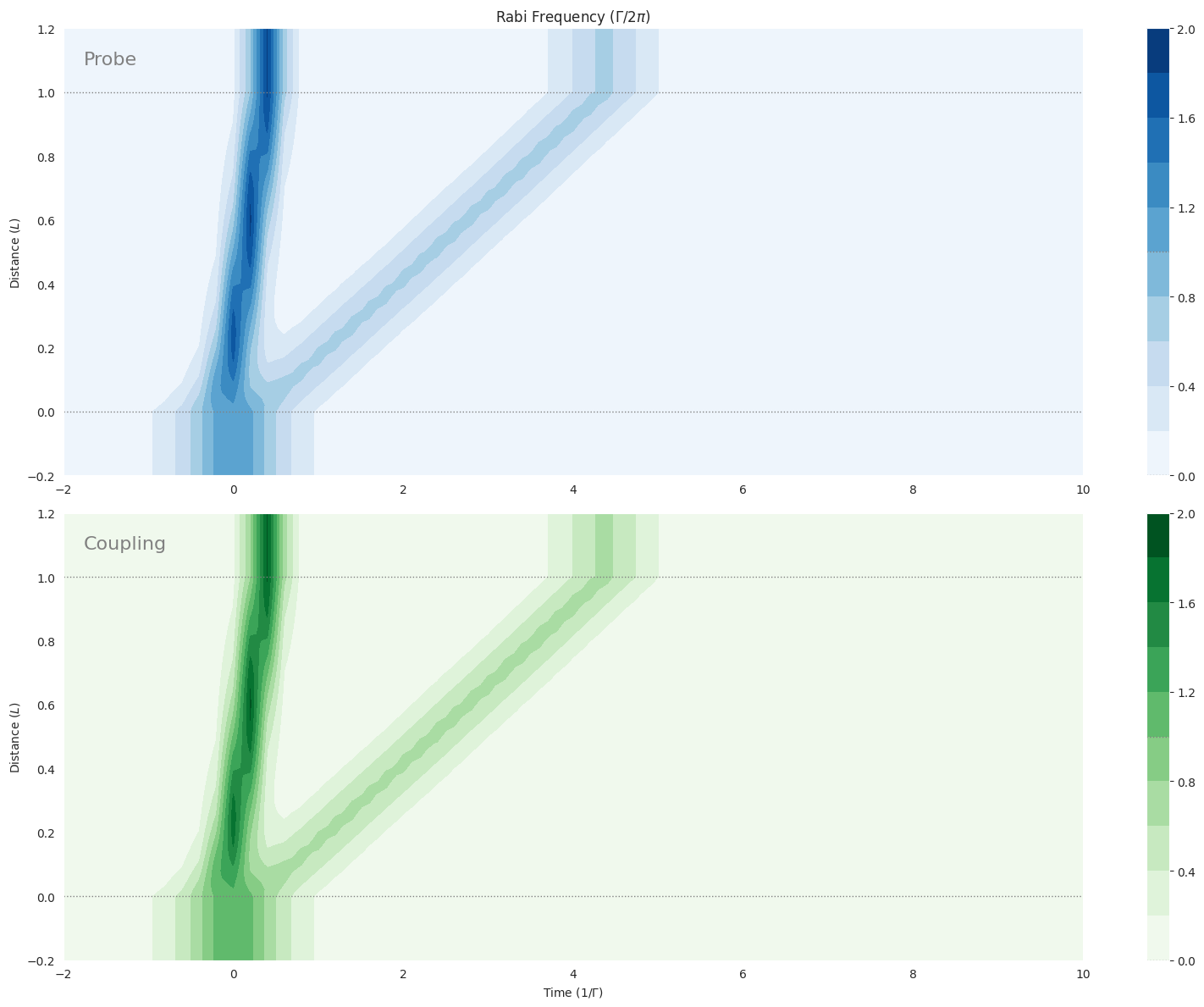
fig = plt.figure(1, figsize=(16, 12))

# Probe
ax = fig.add_subplot(211)
cmap_range = np.linspace(0.0, 2.0, 11)
cf = ax.contourf(
    mb_solve_00.tlist,
    mb_solve_00.zlist,
    np.abs(mb_solve_00.Omegas_zt[0] / (2 * np.pi)),
    cmap_range,
    cmap=plt.cm.Blues,
)
ax.set_title(r"Rabi Frequency ($\Gamma / 2\pi $)")
ax.set_ylabel("Distance ($L$)")
ax.text(
    0.02,
    0.95,
    "Probe",
    verticalalignment="top",
    horizontalalignment="left",
    transform=ax.transAxes,
    color="grey",
    fontsize=16,
)
plt.colorbar(cf)

# Coupling
ax = fig.add_subplot(212)
cmap_range = np.linspace(0.0, 2.0, 11)
cf = ax.contourf(
    mb_solve_00.tlist,
    mb_solve_00.zlist,
    np.abs(mb_solve_00.Omegas_zt[1] / (2 * np.pi)),
    cmap_range,
    cmap=plt.cm.Greens,
)
ax.set_xlabel(r"Time ($1/\Gamma$)")
ax.set_ylabel("Distance ($L$)")
ax.text(
    0.02,
    0.95,
    "Coupling",
    verticalalignment="top",
    horizontalalignment="left",
    transform=ax.transAxes,
    color="grey",
    fontsize=16,
)
plt.colorbar(cf)

# Both
for ax in fig.axes:
    for y in [0.0, 1.0]:
        ax.axhline(y, c="grey", lw=1.0, ls="dotted")
plt.tight_layout()

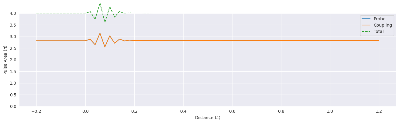
total_area = np.sqrt(
    mb_solve_00.fields_area()[0] ** 2 + mb_solve_00.fields_area()[1] ** 2
)

fig, ax = plt.subplots(figsize=(16, 4))
ax.plot(
    mb_solve_00.zlist,
    mb_solve_00.fields_area()[0] / np.pi,
    label="Probe",
    clip_on=False,
)
ax.plot(
    mb_solve_00.zlist,
    mb_solve_00.fields_area()[1] / np.pi,
    label="Coupling",
    clip_on=False,
)
ax.plot(
    mb_solve_00.zlist, total_area / np.pi, label="Total", ls="dashed", clip_on=False
)
ax.legend()
ax.set_ylim([0.0, 4.0])
ax.set_xlabel("Distance ($L$)")
ax.set_ylabel(r"Pulse Area ($\pi$)");