Λ-Type Three-Level: EIT, Slow Light and Storage
In the Λ-type three-level system a weak probe field couples the ground state |0⟩ to the excited state |1⟩, and a strong coupling field couples |1⟩ to a second ground state |2⟩. When the two-photon resonance condition is met, quantum interference between the two excitation pathways suppresses absorption of the probe — electromagnetically induced transparency (EIT).
Inside the EIT window the probe propagates with a greatly reduced group velocity \(v_g \ll c\), compressing the pulse spatially by the same factor. Adiabatically switching the coupling field off traps the probe as a spin-wave coherence; switching it back on retrieves the pulse — light storage.
This notebook demonstrates:
No coupling — probe absorbed as in a two-level medium.
With coupling — EIT transparency and slow light.
Gaussian atom cloud — slow light and spatial pulse compression.
Light storage and retrieval — coupling switched off then on.
[1]:
import numpy as np
import matplotlib.pyplot as plt
%matplotlib inline
import seaborn as sns

from maxwellbloch import mb_solve

sns.set_style("darkgrid")
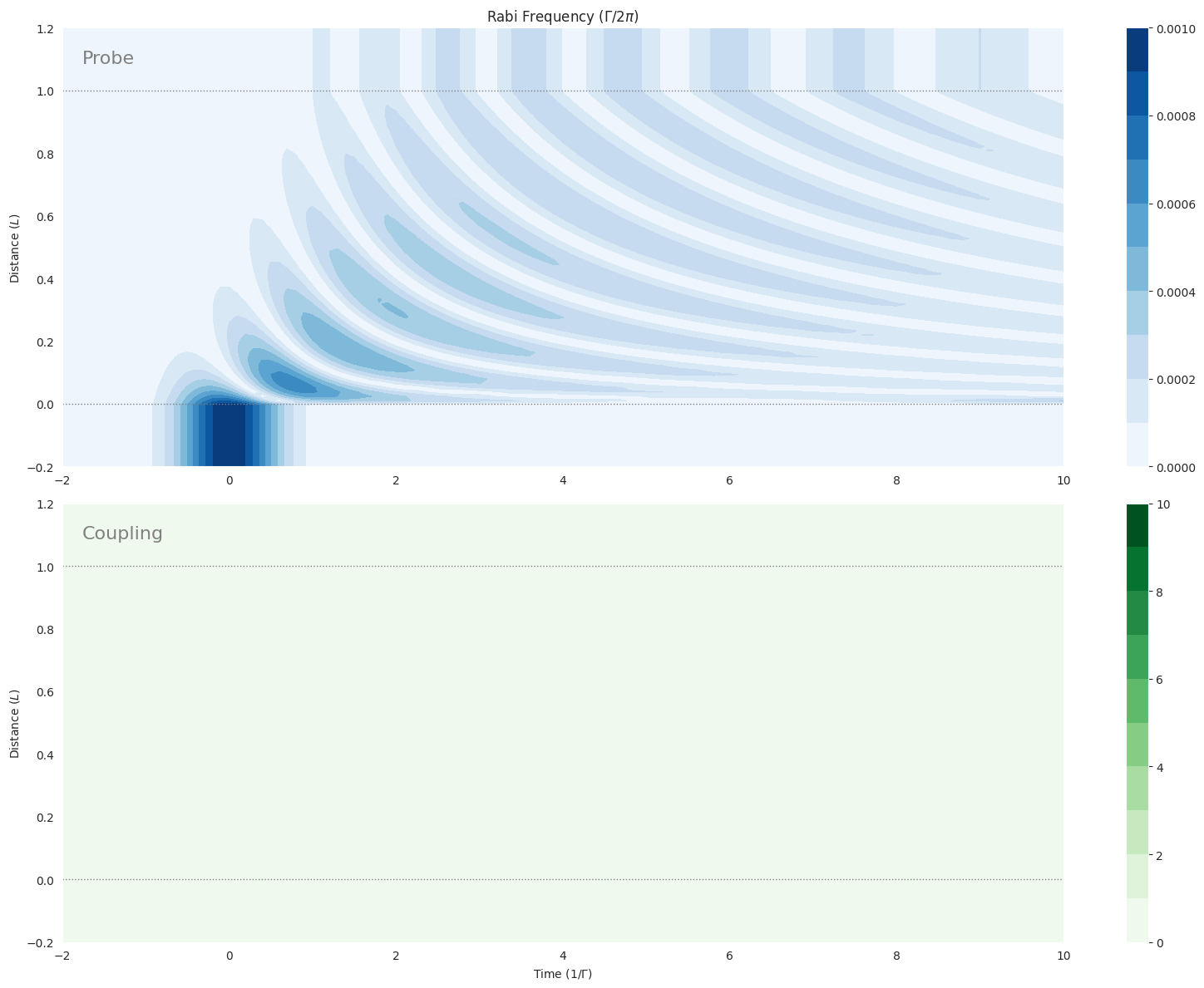
No coupling — resonant absorption
With the coupling field amplitude set to zero the Λ system reduces to a two-level atom. The weak Gaussian probe (\(\Omega_0 = 10^{-3}\,\Gamma\)) is resonantly absorbed as it propagates through the dense medium.
[2]:
mb_solve_json_no_coupling = """
{
  "atom": {
    "fields": [
      {
        "coupled_levels": [[0, 1]],
        "detuning": 0.0,
        "detuning_positive": true,
        "label": "probe",
        "rabi_freq": 1.0e-3,
        "rabi_freq_t_args": {"ampl": 1.0, "centre": 0.0, "fwhm": 1.0},
        "rabi_freq_t_func": "gaussian"
      },
      {
        "coupled_levels": [[1, 2]],
        "detuning": 0.0,
        "detuning_positive": false,
        "label": "coupling",
        "rabi_freq": 0.0,
        "rabi_freq_t_args": {"ampl": 1.0, "fwhm": 0.2, "on": -1.0, "off": 9.0},
        "rabi_freq_t_func": "ramp_onoff"
      }
    ],
    "num_states": 3
  },
  "t_min": -2.0,
  "t_max": 10.0,
  "t_steps": 120,
  "z_min": -0.2,
  "z_max": 1.2,
  "z_steps": 100,
  "z_steps_inner": 2,
  "interaction_strengths": [10.0, 10.0],
  "savefile": "mbs-lambda-weak-pulse-more-atoms-no-coupling"
}
"""

mbs_no_coupling = mb_solve.MBSolve().from_json_str(mb_solve_json_no_coupling)
mbs_no_coupling.mbsolve(recalc=False);
100%|██████████| 100/100 [00:01<00:00, 72.06z/s, Ω_max=0.00154]
Saving MBSolve to mbs-lambda-weak-pulse-more-atoms-no-coupling.qu
[3]:
fig = plt.figure(figsize=(16, 12))

ax = fig.add_subplot(211)
cf = ax.contourf(mbs_no_coupling.tlist, mbs_no_coupling.zlist,
                 np.abs(mbs_no_coupling.Omegas_zt[0] / (2 * np.pi)),
                 np.linspace(0.0, 1.0e-3, 11), cmap=plt.cm.Blues)
ax.set_title(r"Rabi Frequency ($\Gamma / 2\pi$)")
ax.set_ylabel("Distance ($L$)")
ax.text(0.02, 0.95, "Probe", va="top", ha="left", transform=ax.transAxes, color="grey", fontsize=16)
plt.colorbar(cf)
for y in [0.0, 1.0]:
    ax.axhline(y, c="grey", lw=1.0, ls="dotted")

ax = fig.add_subplot(212)
cf = ax.contourf(mbs_no_coupling.tlist, mbs_no_coupling.zlist,
                 np.abs(mbs_no_coupling.Omegas_zt[1] / (2 * np.pi)),
                 np.linspace(0.0, 10.0, 11), cmap=plt.cm.Greens)
ax.set_xlabel(r"Time ($1/\Gamma$)")
ax.set_ylabel("Distance ($L$)")
ax.text(0.02, 0.95, "Coupling", va="top", ha="left", transform=ax.transAxes, color="grey", fontsize=16)
plt.colorbar(cf)
for y in [0.0, 1.0]:
    ax.axhline(y, c="grey", lw=1.0, ls="dotted")

plt.tight_layout()
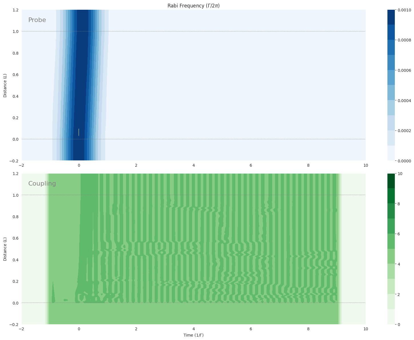
With coupling — EIT transparency and slow light
Switching the coupling on (\(\Omega_c = 5\,\Gamma\)) opens a narrow transparency window at two-photon resonance. The probe now passes through the medium with only a small reduction in amplitude, but its group velocity is greatly reduced — it arrives significantly later than a pulse propagating in vacuum would.
[4]:
mb_solve_json_with_coupling = """
{
  "atom": {
    "fields": [
      {
        "coupled_levels": [[0, 1]],
        "detuning": 0.0,
        "detuning_positive": true,
        "label": "probe",
        "rabi_freq": 1.0e-3,
        "rabi_freq_t_args": {"ampl": 1.0, "centre": 0.0, "fwhm": 1.0},
        "rabi_freq_t_func": "gaussian"
      },
      {
        "coupled_levels": [[1, 2]],
        "detuning": 0.0,
        "detuning_positive": false,
        "label": "coupling",
        "rabi_freq": 5.0,
        "rabi_freq_t_args": {"ampl": 1.0, "fwhm": 0.2, "on": -1.0, "off": 9.0},
        "rabi_freq_t_func": "ramp_onoff"
      }
    ],
    "num_states": 3
  },
  "t_min": -2.0,
  "t_max": 10.0,
  "t_steps": 120,
  "z_min": -0.2,
  "z_max": 1.2,
  "z_steps": 100,
  "z_steps_inner": 2,
  "interaction_strengths": [10.0, 10.0],
  "savefile": "mbs-lambda-weak-pulse-more-atoms-with-coupling"
}
"""

mbs_with_coupling = mb_solve.MBSolve().from_json_str(mb_solve_json_with_coupling)
mbs_with_coupling.mbsolve(recalc=False);
100%|██████████| 100/100 [00:01<00:00, 52.34z/s, Ω_max=31.4]
Saving MBSolve to mbs-lambda-weak-pulse-more-atoms-with-coupling.qu
[5]:
fig = plt.figure(figsize=(16, 12))

ax = fig.add_subplot(211)
cf = ax.contourf(mbs_with_coupling.tlist, mbs_with_coupling.zlist,
                 np.abs(mbs_with_coupling.Omegas_zt[0] / (2 * np.pi)),
                 np.linspace(0.0, 1.0e-3, 11), cmap=plt.cm.Blues)
ax.set_title(r"Rabi Frequency ($\Gamma / 2\pi$)")
ax.set_ylabel("Distance ($L$)")
ax.text(0.02, 0.95, "Probe", va="top", ha="left", transform=ax.transAxes, color="grey", fontsize=16)
plt.colorbar(cf)
for y in [0.0, 1.0]:
    ax.axhline(y, c="grey", lw=1.0, ls="dotted")

ax = fig.add_subplot(212)
cf = ax.contourf(mbs_with_coupling.tlist, mbs_with_coupling.zlist,
                 np.abs(mbs_with_coupling.Omegas_zt[1] / (2 * np.pi)),
                 np.linspace(0.0, 10.0, 11), cmap=plt.cm.Greens)
ax.set_xlabel(r"Time ($1/\Gamma$)")
ax.set_ylabel("Distance ($L$)")
ax.text(0.02, 0.95, "Coupling", va="top", ha="left", transform=ax.transAxes, color="grey", fontsize=16)
plt.colorbar(cf)
for y in [0.0, 1.0]:
    ax.axhline(y, c="grey", lw=1.0, ls="dotted")

plt.tight_layout()
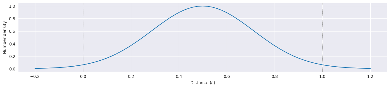
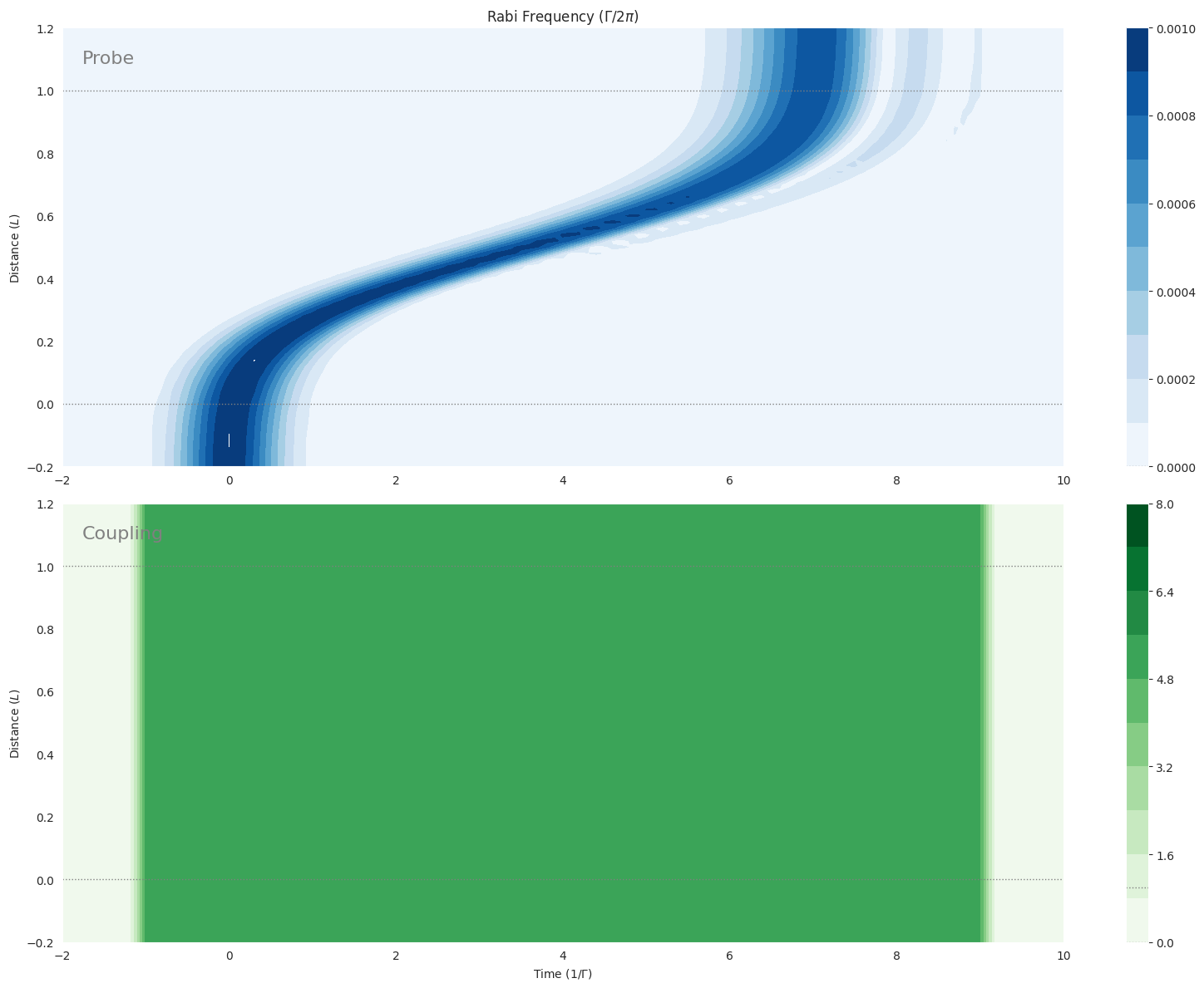
Gaussian atom cloud — slow light and pulse compression
Replacing the uniform medium with a Gaussian density profile makes the slow-light effect spatially inhomogeneous: the probe decelerates as it enters the dense region and reaccelerates as it exits, arriving well after the vacuum transit time.
Because the leading edge of the pulse slows before the trailing edge, the pulse is spatially compressed as it enters the medium — compressed by the same factor \(v_g / c\) by which it is slowed. In EIT experiments with ultracold gases, this compression reduces kilometre-scale pulses to sub-millimetre spatial extent inside the cloud.
[6]:
mb_solve_json_cloud = """
{
  "atom": {
    "fields": [
      {
        "coupled_levels": [[0, 1]],
        "detuning": 0.0,
        "detuning_positive": true,
        "label": "probe",
        "rabi_freq": 1.0e-3,
        "rabi_freq_t_args": {"ampl": 1.0, "centre": 0.0, "fwhm": 1.0},
        "rabi_freq_t_func": "gaussian"
      },
      {
        "coupled_levels": [[1, 2]],
        "detuning": 0.0,
        "detuning_positive": false,
        "label": "coupling",
        "rabi_freq": 5.0,
        "rabi_freq_t_args": {"ampl": 1.0, "fwhm": 0.2, "on": -1.0, "off": 9.0},
        "rabi_freq_t_func": "ramp_onoff"
      }
    ],
    "num_states": 3
  },
  "t_min": -2.0,
  "t_max": 10.0,
  "t_steps": 120,
  "z_min": -0.2,
  "z_max": 1.2,
  "z_steps": 70,
  "z_steps_inner": 100,
  "num_density_z_func": "gaussian",
  "num_density_z_args": {"ampl": 1.0, "fwhm": 0.5, "centre": 0.5},
  "interaction_strengths": [1.0e3, 1.0e3],
  "savefile": "mbs-lambda-weak-pulse-cloud-atoms-some-coupling"
}
"""

mbs_cloud = mb_solve.MBSolve().from_json_str(mb_solve_json_cloud)
[7]:
fig, ax = plt.subplots(figsize=(16, 3))
ax.plot(mbs_cloud.zlist, mbs_cloud.num_density_z_func(mbs_cloud.zlist, mbs_cloud.num_density_z_args))
ax.set_xlabel("Distance ($L$)")
ax.set_ylabel("Number density")
for y_val in [0.0, 1.0]:
    ax.axvline(y_val, c="grey", lw=1.0, ls="dotted");
[8]:
mbs_cloud.mbsolve(recalc=False);
/home/docs/checkouts/readthedocs.org/user_builds/maxwellbloch/envs/v0.12.0/lib/python3.11/site-packages/maxwellbloch/mb_solve.py:344: UserWarning: Savefile was built with maxwellbloch==0.10.0, current version is 0.12.0.
  self.load_results()
[9]:
fig = plt.figure(figsize=(16, 12))

ax = fig.add_subplot(211)
cf = ax.contourf(mbs_cloud.tlist, mbs_cloud.zlist,
                 np.abs(mbs_cloud.Omegas_zt[0] / (2 * np.pi)),
                 np.linspace(0.0, 1.0e-3, 11), cmap=plt.cm.Blues)
ax.set_title(r"Rabi Frequency ($\Gamma / 2\pi$)")
ax.set_ylabel("Distance ($L$)")
ax.text(0.02, 0.95, "Probe", va="top", ha="left", transform=ax.transAxes, color="grey", fontsize=16)
plt.colorbar(cf)

ax = fig.add_subplot(212)
cf = ax.contourf(mbs_cloud.tlist, mbs_cloud.zlist,
                 np.abs(mbs_cloud.Omegas_zt[1] / (2 * np.pi)),
                 np.linspace(0.0, 8.0, 11), cmap=plt.cm.Greens)
ax.set_xlabel(r"Time ($1/\Gamma$)")
ax.set_ylabel("Distance ($L$)")
ax.text(0.02, 0.95, "Coupling", va="top", ha="left", transform=ax.transAxes, color="grey", fontsize=16)
plt.colorbar(cf)

for ax in fig.axes:
    for y in [0.0, 1.0]:
        ax.axhline(y, c="grey", lw=1.0, ls="dotted")
plt.tight_layout()
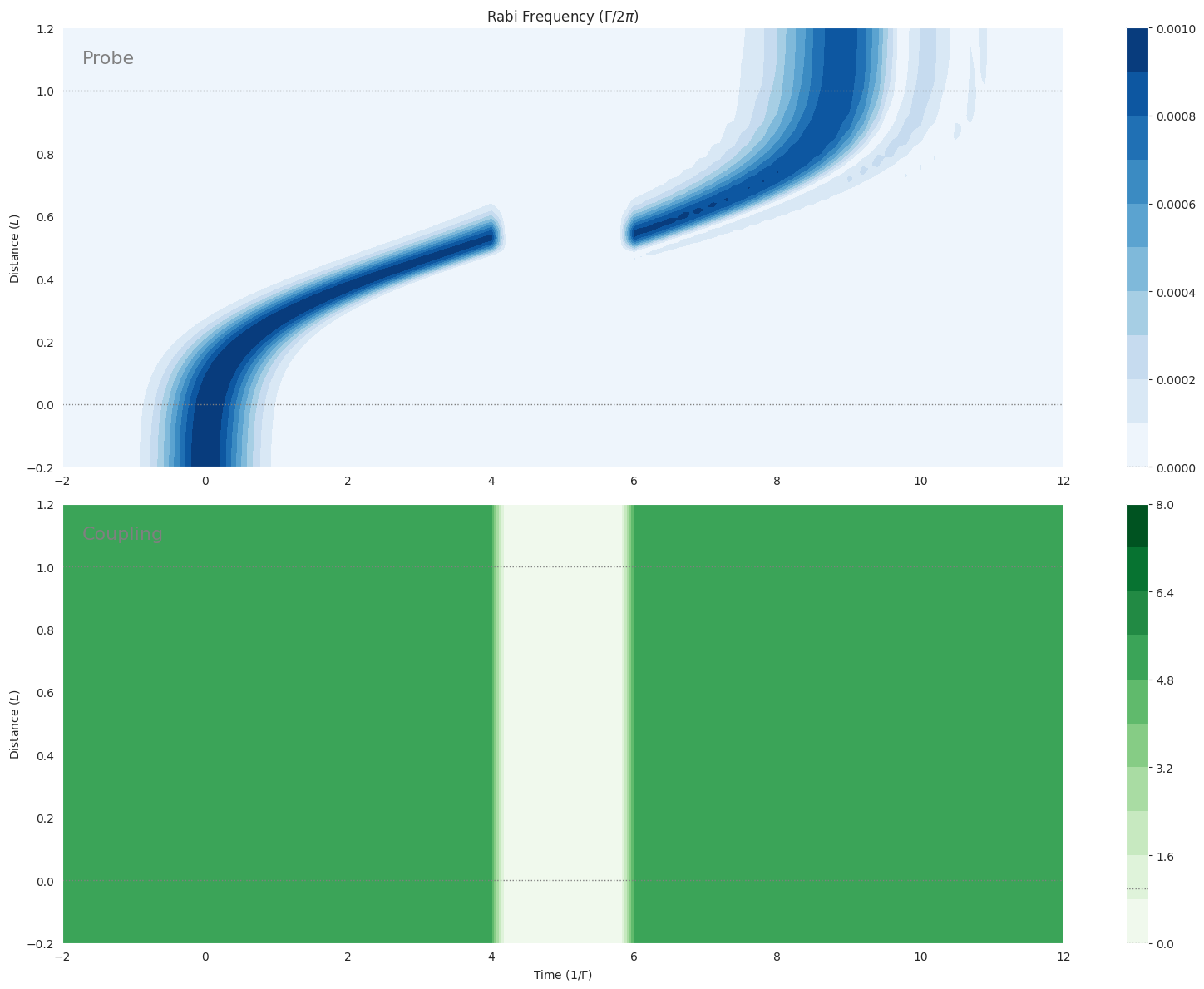
Light storage and retrieval
The coupling field is now switched off at \(t = 4\) (once the probe is inside the cloud) and switched back on at \(t = 6\). Ramping the coupling to zero rotates the dark-state mixing angle to \(\theta \to \pi/2\), mapping the probe coherently onto a long-lived spin-wave excitation of the medium. Restoring the coupling reverses the rotation and the probe re-emerges with its original profile.
Note: this is the most computationally expensive case in this notebook (140 × 50 inner steps). On older hardware it can take several hours.
[10]:
mb_solve_json_store = """
{
  "atom": {
    "fields": [
      {
        "coupled_levels": [[0, 1]],
        "detuning": 0.0,
        "label": "probe",
        "rabi_freq": 1.0e-3,
        "rabi_freq_t_args": {"ampl": 1.0, "centre": 0.0, "fwhm": 1.0},
        "rabi_freq_t_func": "gaussian"
      },
      {
        "coupled_levels": [[1, 2]],
        "detuning": 0.0,
        "detuning_positive": false,
        "label": "coupling",
        "rabi_freq": 5.0,
        "rabi_freq_t_args": {"ampl": 1.0, "fwhm": 0.2, "off": 4.0, "on": 6.0},
        "rabi_freq_t_func": "ramp_offon"
      }
    ],
    "num_states": 3
  },
  "t_min": -2.0,
  "t_max": 12.0,
  "t_steps": 140,
  "z_min": -0.2,
  "z_max": 1.2,
  "z_steps": 140,
  "z_steps_inner": 50,
  "num_density_z_func": "gaussian",
  "num_density_z_args": {"ampl": 1.0, "fwhm": 0.5, "centre": 0.5},
  "interaction_strengths": [1.0e3, 1.0e3],
  "savefile": "mbs-lambda-weak-pulse-cloud-atoms-some-coupling-store"
}
"""

mbs_store = mb_solve.MBSolve().from_json_str(mb_solve_json_store)
mbs_store.mbsolve(recalc=False);
[11]:
fig = plt.figure(figsize=(16, 12))

ax = fig.add_subplot(211)
cf = ax.contourf(mbs_store.tlist, mbs_store.zlist,
                 np.abs(mbs_store.Omegas_zt[0] / (2 * np.pi)),
                 np.linspace(0.0, 1.0e-3, 11), cmap=plt.cm.Blues)
ax.set_title(r"Rabi Frequency ($\Gamma / 2\pi$)")
ax.set_ylabel("Distance ($L$)")
ax.text(0.02, 0.95, "Probe", va="top", ha="left", transform=ax.transAxes, color="grey", fontsize=16)
plt.colorbar(cf)

ax = fig.add_subplot(212)
cf = ax.contourf(mbs_store.tlist, mbs_store.zlist,
                 np.abs(mbs_store.Omegas_zt[1] / (2 * np.pi)),
                 np.linspace(0.0, 8.0, 11), cmap=plt.cm.Greens)
ax.set_xlabel(r"Time ($1/\Gamma$)")
ax.set_ylabel("Distance ($L$)")
ax.text(0.02, 0.95, "Coupling", va="top", ha="left", transform=ax.transAxes, color="grey", fontsize=16)
plt.colorbar(cf)

for ax in fig.axes:
    for y in [0.0, 1.0]:
        ax.axhline(y, c="grey", lw=1.0, ls="dotted")
plt.tight_layout()