V-Type Three-Level: Simultons
In the V-type three-level system a probe field couples the ground state |0⟩ to |1⟩ and a coupling field couples the same ground state to |2⟩. Because both fields share the ground state, they interact through the common atomic coherence.
When the combined pulse area satisfies the V-system area theorem,
the two fields lock into shape-preserving simulton solutions that propagate without absorption — the vector generalisation of the SIT soliton.
This notebook surveys the main regimes:
Weak simulton (0.5π + 0.5π): total area below threshold — both fields absorbed.
Simulton propagation (0.5π + 1.5π): sub-threshold redistribution between fields.
√2π simulton (√2π + √2π): threshold simulton — minimum area for lossless propagation.
√8π soliton formation (√8π + √8π): two-soliton simulton.
Soliton collision: two time-displaced solitons merge into a simulton.
Optical surfer: weak CW probe dragged forward by a 2π coupling soliton.
Double optical surfer: weak CW probe driven by a 4π coupling soliton.
[1]:
import numpy as np
import matplotlib.pyplot as plt
%matplotlib inline
import seaborn as sns

from maxwellbloch import mb_solve

sns.set_style("darkgrid")

sech_fwhm_conv = 1.0 / 2.6339157938
t_width = 1.0 * sech_fwhm_conv  # [τ]
Weak simulton — 0.5π + 0.5π
With both probe and coupling carrying area 0.5π each, the combined area \(\theta_\mathrm{total} = \sqrt{(0.5\pi)^2 + (0.5\pi)^2} \approx 0.71\pi < 2\pi\). This is below the simulton threshold so the medium absorbs both fields — neither propagates as a soliton and the total area decreases monotonically.
[2]:
n = 0.5
ampl_0505 = n / t_width / (2 * np.pi)

mb_solve_json_0505 = """
{
  "atom": {
    "fields": [
      {
        "coupled_levels": [[0, 1]],
        "detuning": 0.0,
        "detuning_positive": true,
        "label": "probe",
        "rabi_freq": 0.20960035913554168,
        "rabi_freq_t_args": {"ampl": 1.0, "centre": 0.0, "width": 0.3796628587572578},
        "rabi_freq_t_func": "sech"
      },
      {
        "coupled_levels": [[0, 2]],
        "detuning": 0.0,
        "detuning_positive": true,
        "label": "coupling",
        "rabi_freq": 0.20960035913554168,
        "rabi_freq_t_args": {"ampl": 1.0, "centre": 0.0, "width": 0.3796628587572578},
        "rabi_freq_t_func": "sech"
      }
    ],
    "num_states": 3
  },
  "t_min": -2.0,
  "t_max": 10.0,
  "t_steps": 60,
  "z_min": -0.2,
  "z_max": 1.2,
  "z_steps": 70,
  "z_steps_inner": 2,
  "interaction_strengths": [10.0, 10.0],
  "savefile": "mbs-vee-sech-0.5pi-0.5pi"
}
"""

mbs_0505 = mb_solve.MBSolve().from_json_str(mb_solve_json_0505)
mbs_0505.mbsolve(recalc=False);
/home/docs/checkouts/readthedocs.org/user_builds/maxwellbloch/envs/v0.12.0/lib/python3.11/site-packages/maxwellbloch/mb_solve.py:344: UserWarning: Savefile was built with maxwellbloch==0.10.0, current version is 0.12.0.
  self.load_results()
[3]:
fig = plt.figure(figsize=(16, 12))
cmap_range = np.linspace(0.0, 0.8, 11)

ax = fig.add_subplot(211)
cf = ax.contourf(mbs_0505.tlist, mbs_0505.zlist,
                 np.abs(mbs_0505.Omegas_zt[0] / (2 * np.pi)), cmap_range, cmap=plt.cm.Blues)
ax.set_title(r"Rabi Frequency ($\Gamma / 2\pi$)")
ax.set_ylabel("Distance ($L$)")
ax.text(0.02, 0.95, "Probe", va="top", ha="left", transform=ax.transAxes, color="grey", fontsize=16)
plt.colorbar(cf)

ax = fig.add_subplot(212)
cf = ax.contourf(mbs_0505.tlist, mbs_0505.zlist,
                 np.abs(mbs_0505.Omegas_zt[1] / (2 * np.pi)), cmap_range, cmap=plt.cm.Greens)
ax.set_xlabel(r"Time ($1/\Gamma$)")
ax.set_ylabel("Distance ($L$)")
ax.text(0.02, 0.95, "Coupling", va="top", ha="left", transform=ax.transAxes, color="grey", fontsize=16)
plt.colorbar(cf)

for ax in fig.axes:
    for y in [0.0, 1.0]:
        ax.axhline(y, c="grey", lw=1.0, ls="dotted")
plt.tight_layout()
[4]:
total_area = np.sqrt(mbs_0505.fields_area()[0]**2 + mbs_0505.fields_area()[1]**2)

fig, ax = plt.subplots(figsize=(16, 4))
ax.plot(mbs_0505.zlist, mbs_0505.fields_area()[0] / np.pi, label="Probe", clip_on=False)
ax.plot(mbs_0505.zlist, mbs_0505.fields_area()[1] / np.pi, label="Coupling", clip_on=False)
ax.plot(mbs_0505.zlist, total_area / np.pi, label="Total", ls="dashed", clip_on=False)
ax.legend()
ax.set_ylim([0.0, 2.0])
ax.set_xlabel("Distance ($L$)")
ax.set_ylabel(r"Pulse Area ($\pi$)");
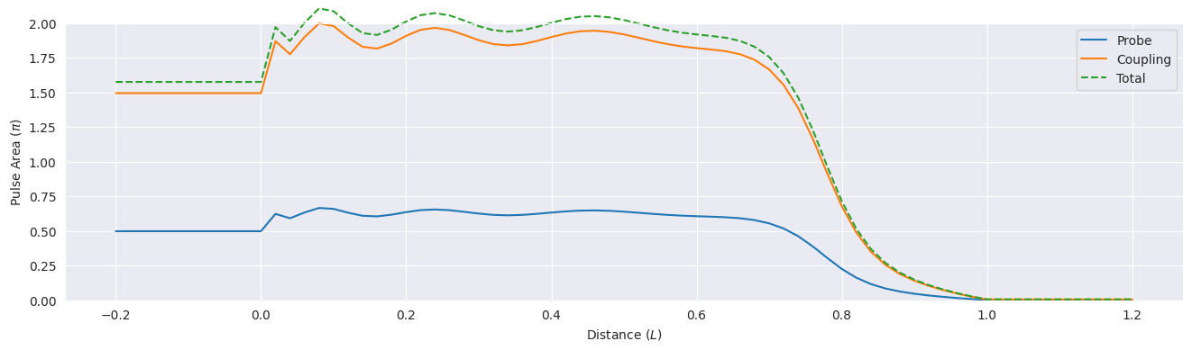
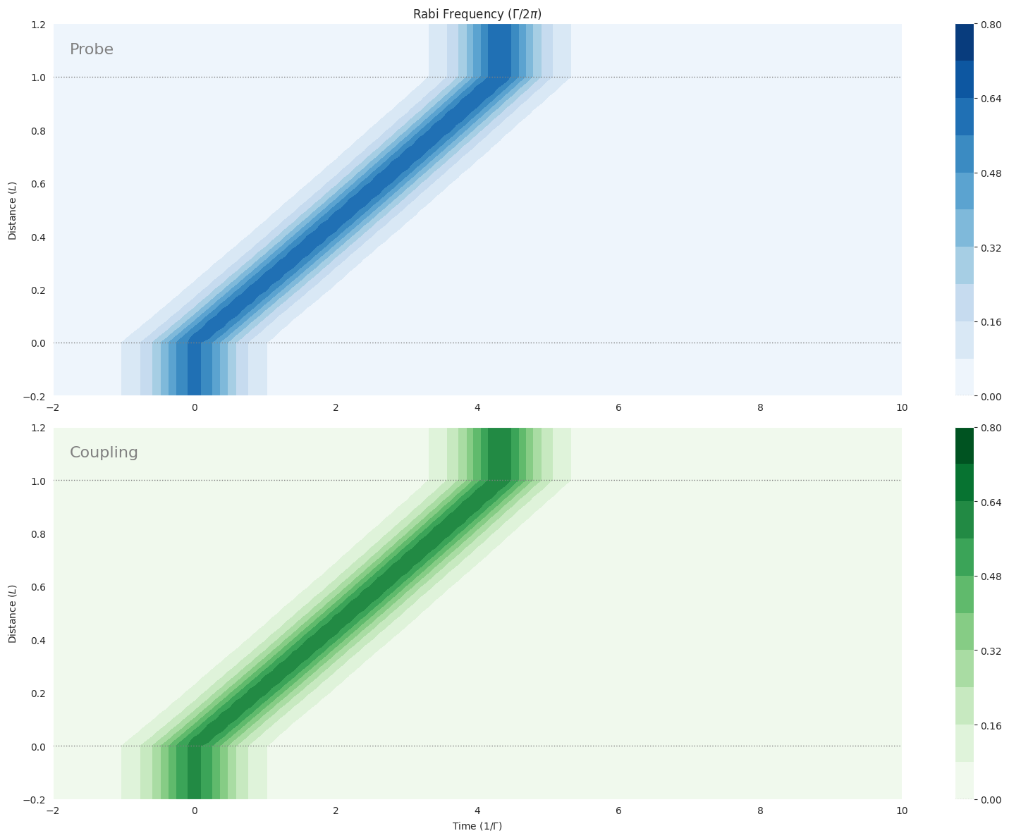
Simulton propagation — 0.5π probe, 1.5π coupling
With probe at 0.5π and coupling at 1.5π the combined area \(\theta_\mathrm{total} = \sqrt{(0.5\pi)^2 + (1.5\pi)^2} \approx 1.58\pi\). Still sub-threshold, but the fields are coupled: the medium redistributes energy from the stronger coupling into the probe as they propagate.
[5]:
ampl_0515_probe = 0.5 / t_width / (2 * np.pi)
ampl_0515_coupling = 1.5 / t_width / (2 * np.pi)

mb_solve_json_0515 = """
{
  "atom": {
    "fields": [
      {
        "coupled_levels": [[0, 1]],
        "detuning": 0.0,
        "detuning_positive": true,
        "label": "probe",
        "rabi_freq": 0.20960035913554168,
        "rabi_freq_t_args": {"ampl": 1.0, "centre": 0.0, "width": 0.3796628587572578},
        "rabi_freq_t_func": "sech"
      },
      {
        "coupled_levels": [[0, 2]],
        "detuning": 0.0,
        "detuning_positive": true,
        "label": "coupling",
        "rabi_freq": 0.628801077406625,
        "rabi_freq_t_args": {"ampl": 1.0, "centre": 0.0, "width": 0.3796628587572578},
        "rabi_freq_t_func": "sech"
      }
    ],
    "num_states": 3
  },
  "t_min": -2.0,
  "t_max": 10.0,
  "t_steps": 60,
  "z_min": -0.2,
  "z_max": 1.2,
  "z_steps": 70,
  "z_steps_inner": 2,
  "interaction_strengths": [10.0, 10.0],
  "savefile": "mb-solve-vee-sech-0.5pi-1.5pi"
}
"""

mbs_0515 = mb_solve.MBSolve().from_json_str(mb_solve_json_0515)
mbs_0515.mbsolve(recalc=False);
[6]:
fig = plt.figure(figsize=(16, 12))
cmap_range = np.linspace(0.0, 0.8, 11)

ax = fig.add_subplot(211)
cf = ax.contourf(mbs_0515.tlist, mbs_0515.zlist,
                 np.abs(mbs_0515.Omegas_zt[0] / (2 * np.pi)), cmap_range, cmap=plt.cm.Blues)
ax.set_title(r"Rabi Frequency ($\Gamma / 2\pi$)")
ax.set_ylabel("Distance ($L$)")
ax.text(0.02, 0.95, "Probe", va="top", ha="left", transform=ax.transAxes, color="grey", fontsize=16)
plt.colorbar(cf)

ax = fig.add_subplot(212)
cf = ax.contourf(mbs_0515.tlist, mbs_0515.zlist,
                 np.abs(mbs_0515.Omegas_zt[1] / (2 * np.pi)), cmap_range, cmap=plt.cm.Greens)
ax.set_xlabel(r"Time ($1/\Gamma$)")
ax.set_ylabel("Distance ($L$)")
ax.text(0.02, 0.95, "Coupling", va="top", ha="left", transform=ax.transAxes, color="grey", fontsize=16)
plt.colorbar(cf)

for ax in fig.axes:
    for y in [0.0, 1.0]:
        ax.axhline(y, c="grey", lw=1.0, ls="dotted")
plt.tight_layout()
[7]:
total_area = np.sqrt(mbs_0515.fields_area()[0]**2 + mbs_0515.fields_area()[1]**2)

fig, ax = plt.subplots(figsize=(16, 4))
ax.plot(mbs_0515.zlist, mbs_0515.fields_area()[0] / np.pi, label="Probe", clip_on=False)
ax.plot(mbs_0515.zlist, mbs_0515.fields_area()[1] / np.pi, label="Coupling", clip_on=False)
ax.plot(mbs_0515.zlist, total_area / np.pi, label="Total", ls="dashed", clip_on=False)
ax.legend()
ax.set_ylim([0.0, 2.0])
ax.set_xlabel("Distance ($L$)")
ax.set_ylabel(r"Pulse Area ($\pi$)");
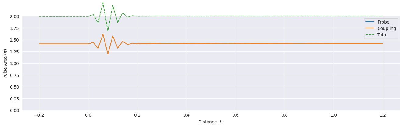
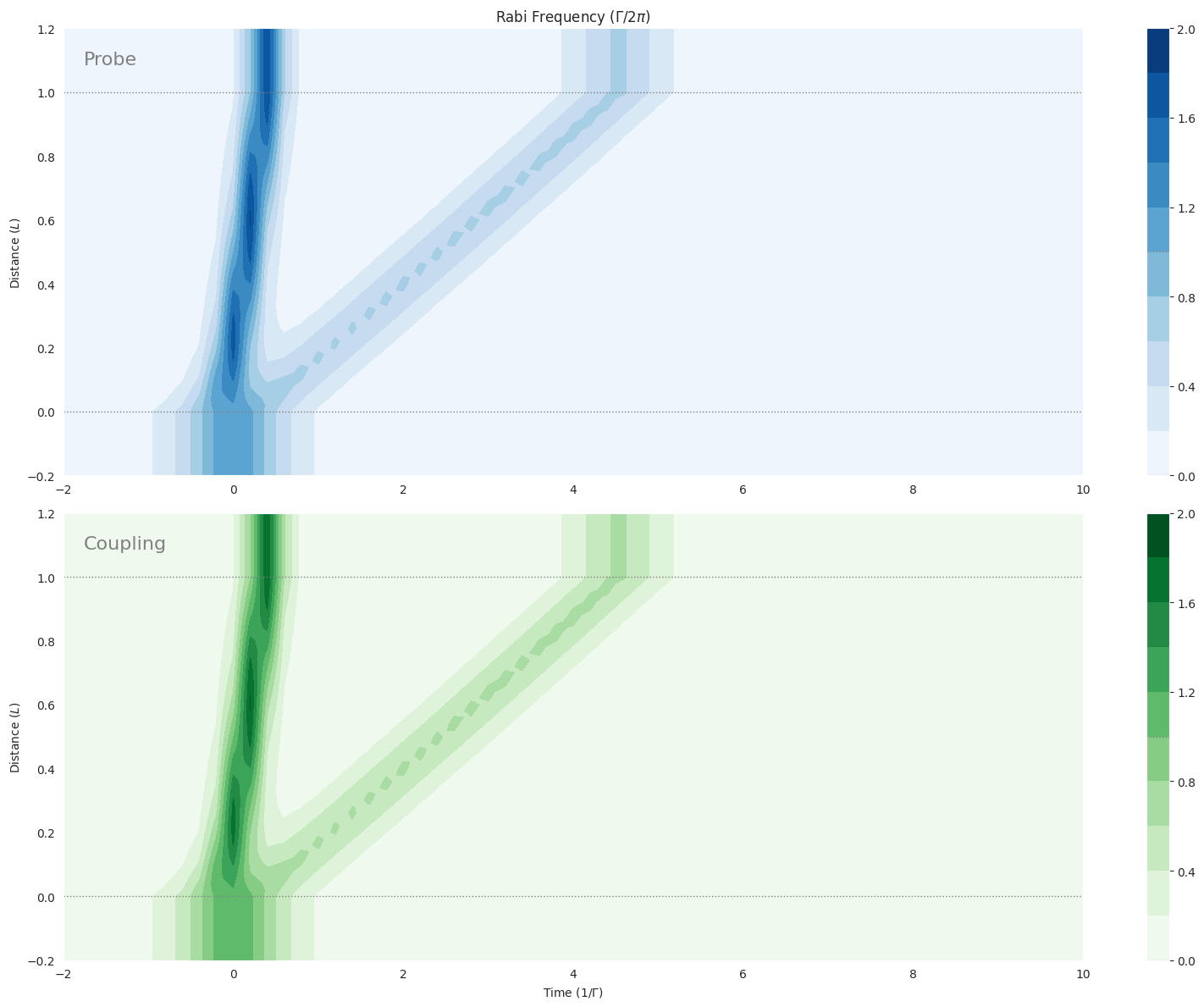
√2π simulton formation
At \(\theta_\mathrm{probe} = \theta_\mathrm{coupling} = \sqrt{2}\pi\) the combined area is exactly \(\theta_\mathrm{total} = \sqrt{2\pi^2 + 2\pi^2} = 2\pi\) — the threshold simulton. Both fields propagate without loss, locked together in shape and velocity.
[8]:
ampl_s2 = np.sqrt(2) / t_width / (2 * np.pi)

mb_solve_json_s2 = """
{
  "atom": {
    "fields": [
      {
        "coupled_levels": [[0, 1]],
        "detuning": 0.0,
        "detuning_positive": true,
        "label": "probe",
        "rabi_freq": 0.592839341136,
        "rabi_freq_t_args": {"ampl": 1.0, "centre": 0.0, "width": 0.3796628587572578},
        "rabi_freq_t_func": "sech"
      },
      {
        "coupled_levels": [[0, 2]],
        "detuning": 0.0,
        "detuning_positive": true,
        "label": "coupling",
        "rabi_freq": 0.592839341136,
        "rabi_freq_t_args": {"ampl": 1.0, "centre": 0.0, "width": 0.3796628587572578},
        "rabi_freq_t_func": "sech"
      }
    ],
    "num_states": 3
  },
  "t_min": -2.0,
  "t_max": 10.0,
  "t_steps": 60,
  "z_min": -0.2,
  "z_max": 1.2,
  "z_steps": 70,
  "z_steps_inner": 1,
  "num_density_z_func": "square",
  "num_density_z_args": {"on": 0.0, "off": 1.0, "ampl": 1.0},
  "interaction_strengths": [10.0, 10.0],
  "savefile": "mbs-vee-sech-sqrt2pi-sqrt2pi"
}
"""

mbs_s2 = mb_solve.MBSolve().from_json_str(mb_solve_json_s2)
mbs_s2.mbsolve(recalc=False);
[9]:
fig = plt.figure(figsize=(16, 12))
cmap_range = np.linspace(0.0, 0.8, 11)

ax = fig.add_subplot(211)
cf = ax.contourf(mbs_s2.tlist, mbs_s2.zlist,
                 np.abs(mbs_s2.Omegas_zt[0] / (2 * np.pi)), cmap_range, cmap=plt.cm.Blues)
ax.set_title(r"Rabi Frequency ($\Gamma / 2\pi$)")
ax.set_ylabel("Distance ($L$)")
ax.text(0.02, 0.95, "Probe", va="top", ha="left", transform=ax.transAxes, color="grey", fontsize=16)
plt.colorbar(cf)

ax = fig.add_subplot(212)
cf = ax.contourf(mbs_s2.tlist, mbs_s2.zlist,
                 np.abs(mbs_s2.Omegas_zt[1] / (2 * np.pi)), cmap_range, cmap=plt.cm.Greens)
ax.set_xlabel(r"Time ($1/\Gamma$)")
ax.set_ylabel("Distance ($L$)")
ax.text(0.02, 0.95, "Coupling", va="top", ha="left", transform=ax.transAxes, color="grey", fontsize=16)
plt.colorbar(cf)

for ax in fig.axes:
    for y in [0.0, 1.0]:
        ax.axhline(y, c="grey", lw=1.0, ls="dotted")
plt.tight_layout()
[10]:
total_area = np.sqrt(mbs_s2.fields_area()[0]**2 + mbs_s2.fields_area()[1]**2)

fig, ax = plt.subplots(figsize=(16, 4))
ax.plot(mbs_s2.zlist, mbs_s2.fields_area()[0] / np.pi, label="Probe", clip_on=False)
ax.plot(mbs_s2.zlist, mbs_s2.fields_area()[1] / np.pi, label="Coupling", clip_on=False)
ax.plot(mbs_s2.zlist, total_area / np.pi, label="Total", ls="dashed", clip_on=False)
ax.legend()
ax.set_ylim([0.0, 2.0])
ax.set_xlabel("Distance ($L$)")
ax.set_ylabel(r"Pulse Area ($\pi$)");
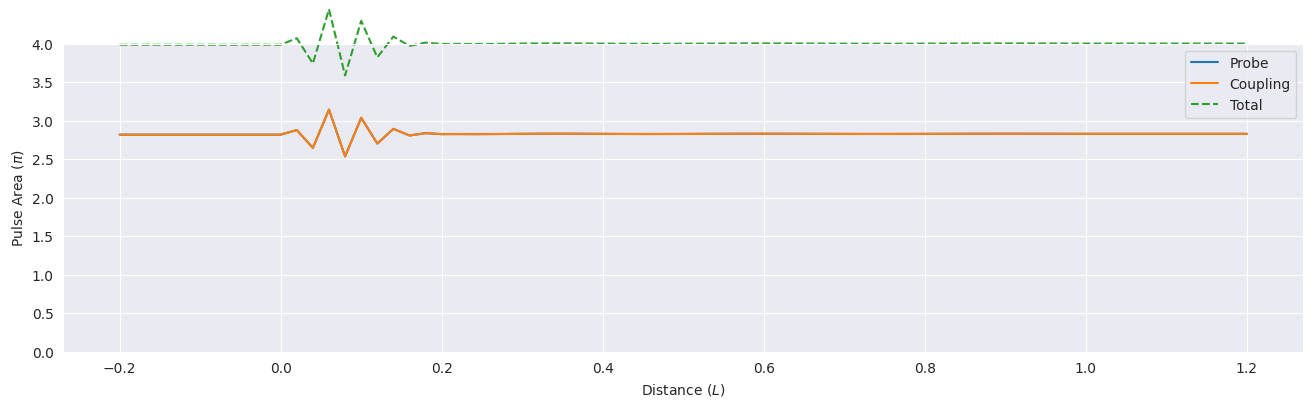
√8π soliton formation
At \(\theta_\mathrm{probe} = \theta_\mathrm{coupling} = \sqrt{8}\pi = 2\sqrt{2}\pi\) the combined area is \(4\pi\), supporting a two-soliton simulton. Each field pulse breaks into two SIT-soliton-like sub-pulses that travel together through the medium.
[11]:
ampl_s8 = np.sqrt(8) / t_width / (2 * np.pi)

mb_solve_json_s8 = """
{
  "atom": {
    "decays": [{"channels": [[0, 1], [0, 2]], "rate": 0.0}],
    "energies": [],
    "fields": [
      {
        "coupled_levels": [[0, 1]],
        "detuning": 0.0,
        "detuning_positive": true,
        "label": "probe",
        "rabi_freq": 1.18567868227,
        "rabi_freq_t_args": {"ampl": 1.0, "centre": 0.0, "width": 0.3796628587572578},
        "rabi_freq_t_func": "sech"
      },
      {
        "coupled_levels": [[0, 2]],
        "detuning": 0.0,
        "detuning_positive": true,
        "label": "coupling",
        "rabi_freq": 1.18567868227,
        "rabi_freq_t_args": {"ampl": 1.0, "centre": 0.0, "width": 0.3796628587572578},
        "rabi_freq_t_func": "sech"
      }
    ],
    "num_states": 3
  },
  "t_min": -2.0,
  "t_max": 10.0,
  "t_steps": 60,
  "z_min": -0.2,
  "z_max": 1.2,
  "z_steps": 70,
  "z_steps_inner": 1,
  "interaction_strengths": [10.0, 10.0],
  "savefile": "mbs-vee-sech-sqrt8pi-sqrt8pi"
}
"""

mbs_s8 = mb_solve.MBSolve().from_json_str(mb_solve_json_s8)
mbs_s8.mbsolve(recalc=False);
[12]:
fig = plt.figure(figsize=(16, 12))
cmap_range = np.linspace(0.0, 2.0, 11)

ax = fig.add_subplot(211)
cf = ax.contourf(mbs_s8.tlist, mbs_s8.zlist,
                 np.abs(mbs_s8.Omegas_zt[0] / (2 * np.pi)), cmap_range, cmap=plt.cm.Blues)
ax.set_title(r"Rabi Frequency ($\Gamma / 2\pi$)")
ax.set_ylabel("Distance ($L$)")
ax.text(0.02, 0.95, "Probe", va="top", ha="left", transform=ax.transAxes, color="grey", fontsize=16)
plt.colorbar(cf)

ax = fig.add_subplot(212)
cf = ax.contourf(mbs_s8.tlist, mbs_s8.zlist,
                 np.abs(mbs_s8.Omegas_zt[1] / (2 * np.pi)), cmap_range, cmap=plt.cm.Greens)
ax.set_xlabel(r"Time ($1/\Gamma$)")
ax.set_ylabel("Distance ($L$)")
ax.text(0.02, 0.95, "Coupling", va="top", ha="left", transform=ax.transAxes, color="grey", fontsize=16)
plt.colorbar(cf)

for ax in fig.axes:
    for y in [0.0, 1.0]:
        ax.axhline(y, c="grey", lw=1.0, ls="dotted")
plt.tight_layout()
[13]:
total_area = np.sqrt(mbs_s8.fields_area()[0]**2 + mbs_s8.fields_area()[1]**2)

fig, ax = plt.subplots(figsize=(16, 4))
ax.plot(mbs_s8.zlist, mbs_s8.fields_area()[0] / np.pi, label="Probe", clip_on=False)
ax.plot(mbs_s8.zlist, mbs_s8.fields_area()[1] / np.pi, label="Coupling", clip_on=False)
ax.plot(mbs_s8.zlist, total_area / np.pi, label="Total", ls="dashed", clip_on=False)
ax.legend()
ax.set_ylim([0.0, 4.0])
ax.set_xlabel("Distance ($L$)")
ax.set_ylabel(r"Pulse Area ($\pi$)");
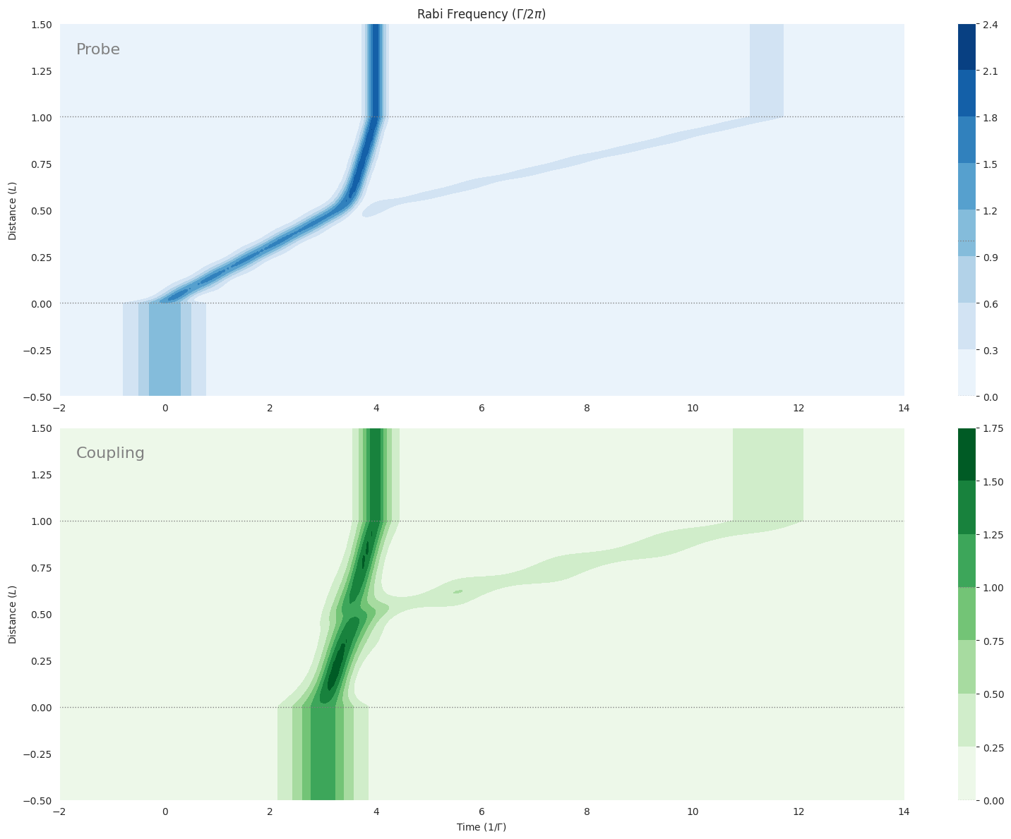
Soliton collision — solitons form simulton
A \(\sqrt{8}\pi\) sech pulse on the probe enters at \(t = 0\); a second \(\sqrt{8}\pi\) sech pulse on the coupling enters at \(t = 3\). In the medium the two pulses interact via the atoms: the collision reshapes both into a shared simulton — demonstrating that solitons can lock together even when launched at different times.
[14]:
ampl_coll = np.sqrt(8) / t_width / (2 * np.pi)

mb_solve_json_coll = """
{{
  "atom": {{
    "fields": [
      {{
        "coupled_levels": [[0, 1]],
        "label": "probe",
        "rabi_freq": 1.0,
        "rabi_freq_t_args": {{"ampl": {ampl_coll}, "centre": 0.0, "width": {t_width}}},
        "rabi_freq_t_func": "sech"
      }},
      {{
        "coupled_levels": [[0, 2]],
        "label": "coupling",
        "rabi_freq": 1.0,
        "rabi_freq_t_args": {{"ampl": {ampl_coll}, "centre": 3.0, "width": {t_width}}},
        "rabi_freq_t_func": "sech"
      }}
    ],
    "num_states": 3
  }},
  "t_min": -2.0,
  "t_max": 14.0,
  "t_steps": 200,
  "z_min": -0.5,
  "z_max": 1.5,
  "z_steps": 500,
  "z_steps_inner": 1,
  "interaction_strengths": [50.0, 10.0],
  "savefile": "mbs-vee-sech-sqrt8pi-sqrt8pi-collision"
}}
""".format(ampl_coll=ampl_coll, t_width=t_width)

mbs_coll = mb_solve.MBSolve().from_json_str(mb_solve_json_coll)
mbs_coll.mbsolve(recalc=False);
[15]:
fig = plt.figure(figsize=(16, 12))

ax = fig.add_subplot(211)
cf = ax.contourf(mbs_coll.tlist, mbs_coll.zlist,
                 np.abs(mbs_coll.Omegas_zt[0] / (2 * np.pi)), cmap=plt.cm.Blues)
ax.set_title(r"Rabi Frequency ($\Gamma / 2\pi$)")
ax.set_ylabel("Distance ($L$)")
ax.text(0.02, 0.95, "Probe", va="top", ha="left", transform=ax.transAxes, color="grey", fontsize=16)
plt.colorbar(cf)

ax = fig.add_subplot(212)
cf = ax.contourf(mbs_coll.tlist, mbs_coll.zlist,
                 np.abs(mbs_coll.Omegas_zt[1] / (2 * np.pi)), cmap=plt.cm.Greens)
ax.set_xlabel(r"Time ($1/\Gamma$)")
ax.set_ylabel("Distance ($L$)")
ax.text(0.02, 0.95, "Coupling", va="top", ha="left", transform=ax.transAxes, color="grey", fontsize=16)
plt.colorbar(cf)

for ax in fig.axes:
    for y in [0.0, 1.0]:
        ax.axhline(y, c="grey", lw=1.0, ls="dotted")
plt.tight_layout()
[16]:
total_area = np.sqrt(mbs_coll.fields_area()[0]**2 + mbs_coll.fields_area()[1]**2)

fig, ax = plt.subplots(figsize=(16, 4))
ax.plot(mbs_coll.zlist, mbs_coll.fields_area()[0] / np.pi, label="Probe", clip_on=False)
ax.plot(mbs_coll.zlist, mbs_coll.fields_area()[1] / np.pi, label="Coupling", clip_on=False)
ax.plot(mbs_coll.zlist, total_area / np.pi, label="Total", ls="dashed", clip_on=False)
ax.legend()
ax.set_ylim([0.0, 4.0])
ax.set_xlabel("Distance ($L$)")
ax.set_ylabel(r"Pulse Area ($\pi$)");
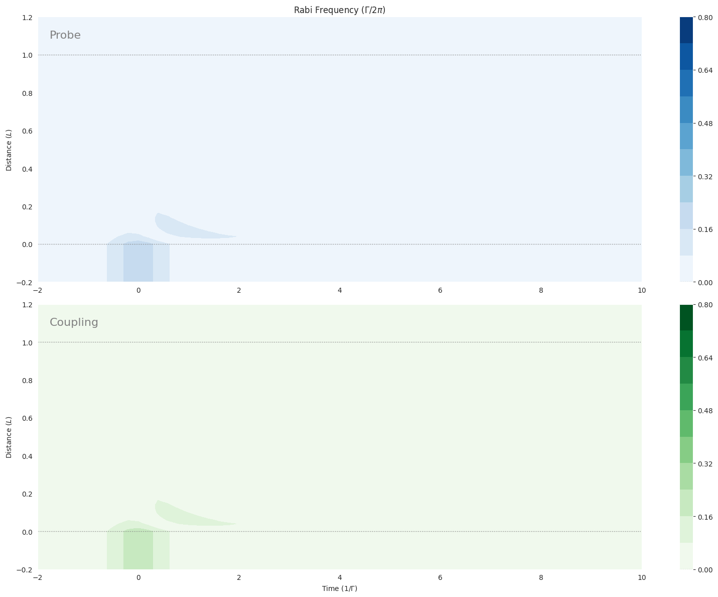
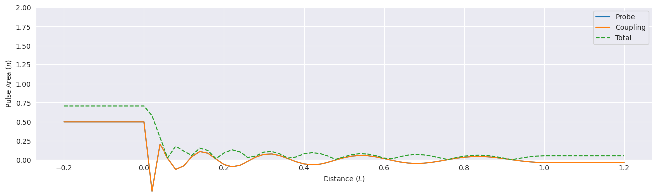
Optical surfer — 2π coupling soliton on CW probe
A weak CW probe (\(\Omega_\mathrm{probe} = 10^{-3}\,\Gamma\)) is ramped on at \(t = -1\). A 2π sech soliton is launched on the coupling field at \(t = 0\). The coupling soliton propagates as a SIT soliton; where it overlaps the probe, it opens a local transparency window that drags the probe forward — an optical surfer riding on the CW background.
[17]:
ampl_surf2 = 2.0 / t_width / (2 * np.pi)

mb_solve_json_surf2 = """
{
  "atom": {
    "fields": [
      {
        "coupled_levels": [[0, 1]],
        "detuning": 0.0,
        "detuning_positive": true,
        "label": "probe",
        "rabi_freq": 1.0e-3,
        "rabi_freq_t_args": {"ampl": 1.0, "on": -1.0, "fwhm": 0.3796628587572578},
        "rabi_freq_t_func": "ramp_on"
      },
      {
        "coupled_levels": [[0, 2]],
        "detuning": 0.0,
        "detuning_positive": true,
        "label": "coupling",
        "rabi_freq": 0.8384014365421667,
        "rabi_freq_t_args": {"ampl": 1.0, "centre": 0.0, "width": 0.3796628587572578},
        "rabi_freq_t_func": "sech"
      }
    ],
    "num_states": 3
  },
  "t_min": -2.0,
  "t_max": 10.0,
  "t_steps": 120,
  "z_min": -0.2,
  "z_max": 1.2,
  "z_steps": 140,
  "z_steps_inner": 2,
  "interaction_strengths": [10.0, 10.0],
  "savefile": "mbs-vee-weak-cw-sech-2pi"
}
"""

mbs_surf2 = mb_solve.MBSolve().from_json_str(mb_solve_json_surf2)
mbs_surf2.mbsolve(recalc=False);
[18]:
fig = plt.figure(figsize=(16, 12))

ax = fig.add_subplot(211)
cf = ax.contourf(mbs_surf2.tlist, mbs_surf2.zlist,
                 np.abs(mbs_surf2.Omegas_zt[0] / (2 * np.pi)),
                 np.linspace(0.0, 2e-3, 11), cmap=plt.cm.Blues)
ax.set_title(r"Rabi Frequency ($\Gamma / 2\pi$)")
ax.set_ylabel("Distance ($L$)")
ax.text(0.02, 0.95, "Probe", va="top", ha="left", transform=ax.transAxes, color="grey", fontsize=16)
plt.colorbar(cf)

ax = fig.add_subplot(212)
cf = ax.contourf(mbs_surf2.tlist, mbs_surf2.zlist,
                 np.abs(mbs_surf2.Omegas_zt[1] / (2 * np.pi)),
                 np.linspace(0.0, 1.0, 11), cmap=plt.cm.Greens)
ax.set_xlabel(r"Time ($1/\Gamma$)")
ax.set_ylabel("Distance ($L$)")
ax.text(0.02, 0.95, "Coupling", va="top", ha="left", transform=ax.transAxes, color="grey", fontsize=16)
plt.colorbar(cf)

for ax in fig.axes:
    for y in [0.0, 1.0]:
        ax.axhline(y, c="grey", lw=1.0, ls="dotted")
plt.tight_layout()
[19]:
total_area = np.sqrt(mbs_surf2.fields_area()[0]**2 + mbs_surf2.fields_area()[1]**2)

fig, ax = plt.subplots(figsize=(16, 4))
ax.plot(mbs_surf2.zlist, mbs_surf2.fields_area()[0] / np.pi, label="Probe", clip_on=False)
ax.plot(mbs_surf2.zlist, mbs_surf2.fields_area()[1] / np.pi, label="Coupling", clip_on=False)
ax.plot(mbs_surf2.zlist, total_area / np.pi, label="Total", ls="dashed", clip_on=False)
ax.legend()
ax.set_ylim([0.0, 2.0])
ax.set_xlabel("Distance ($L$)")
ax.set_ylabel(r"Pulse Area ($\pi$)");
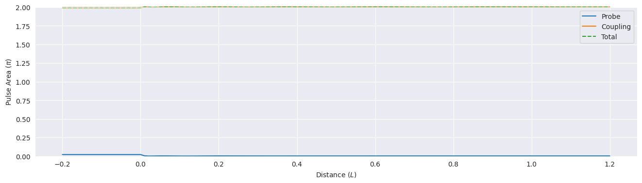
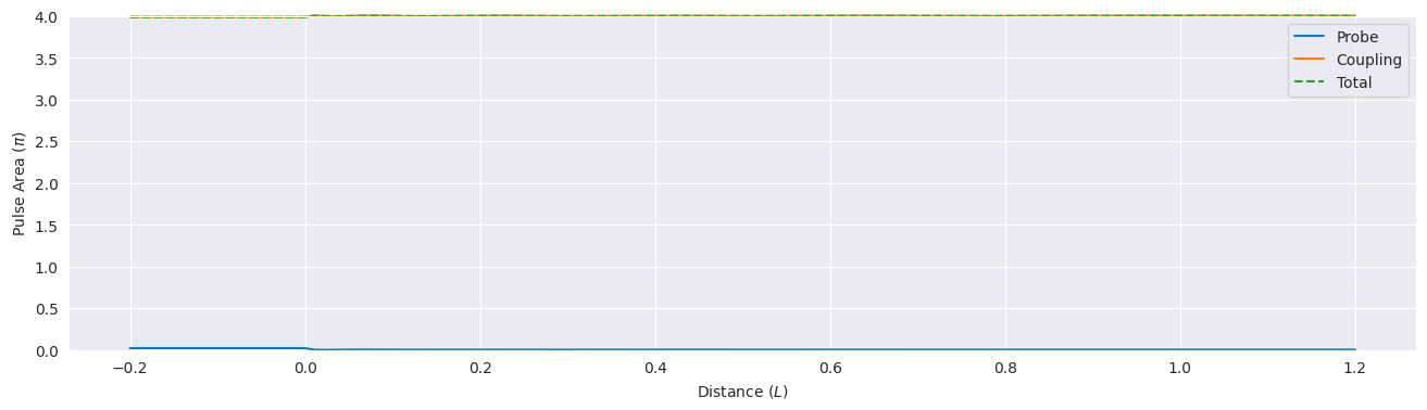
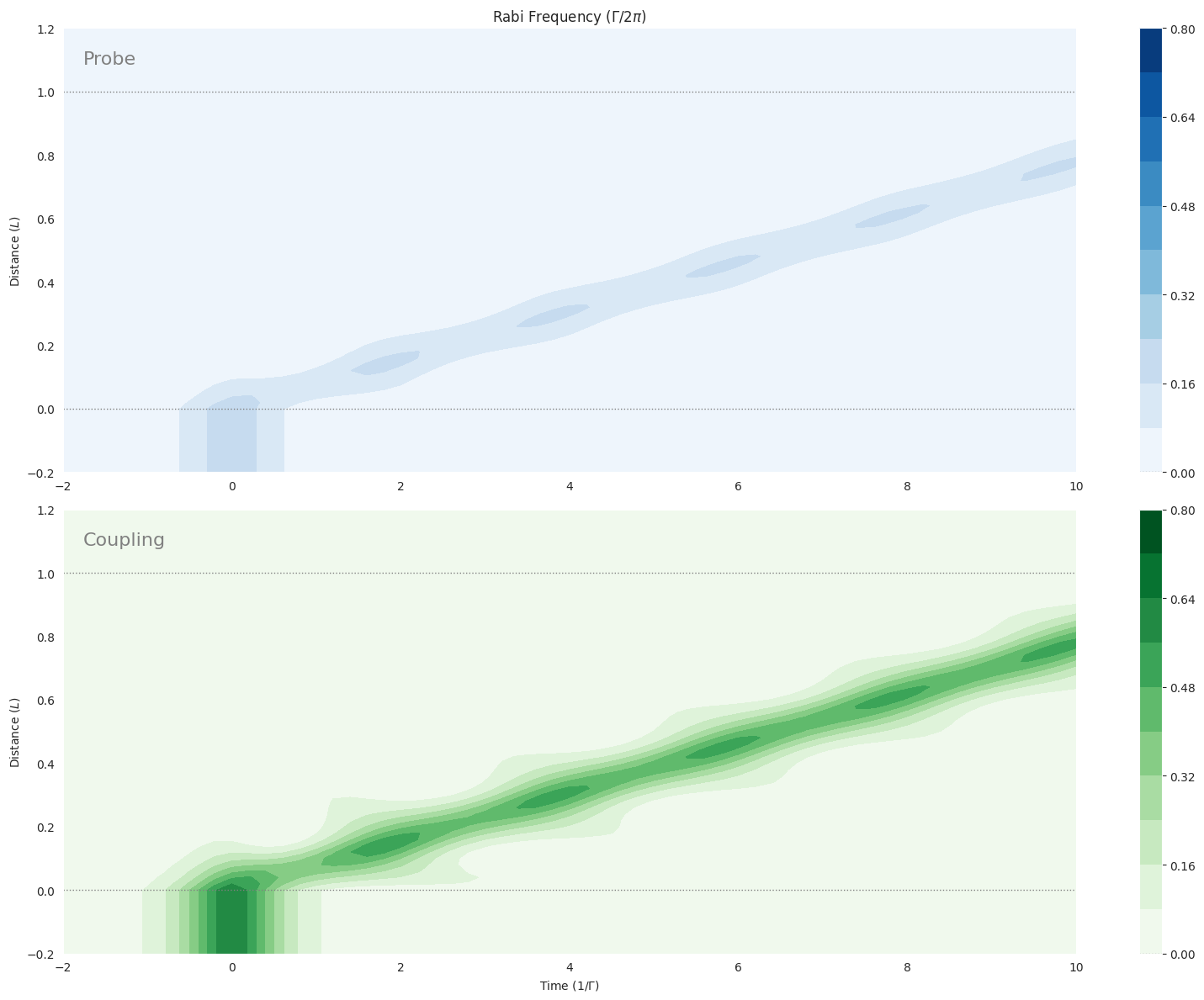
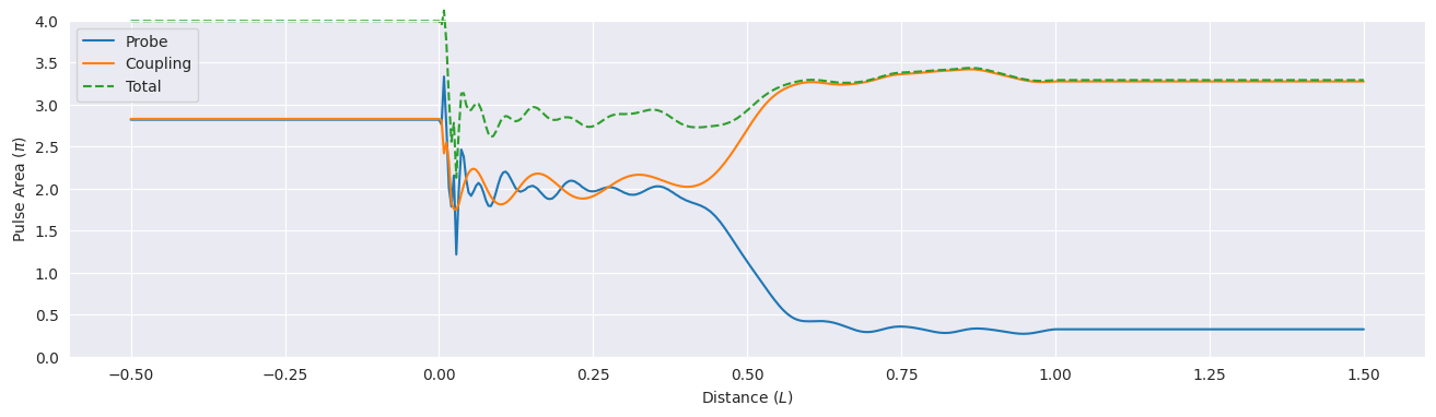
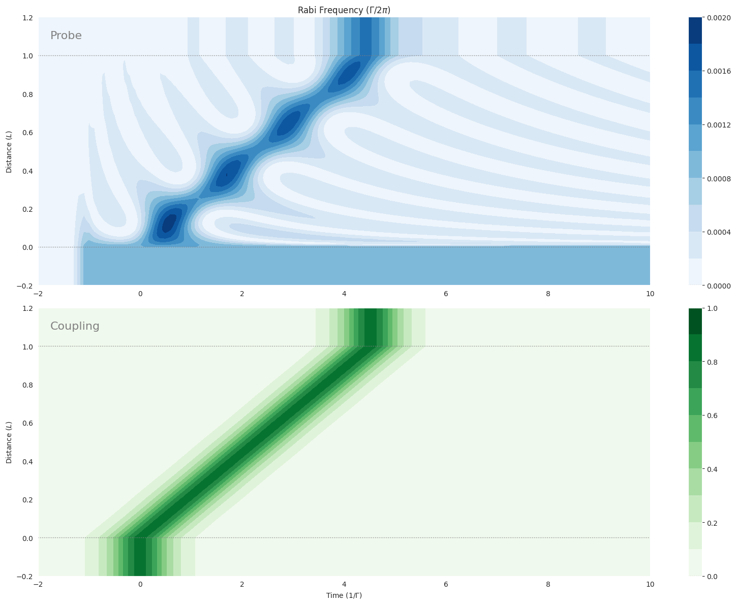
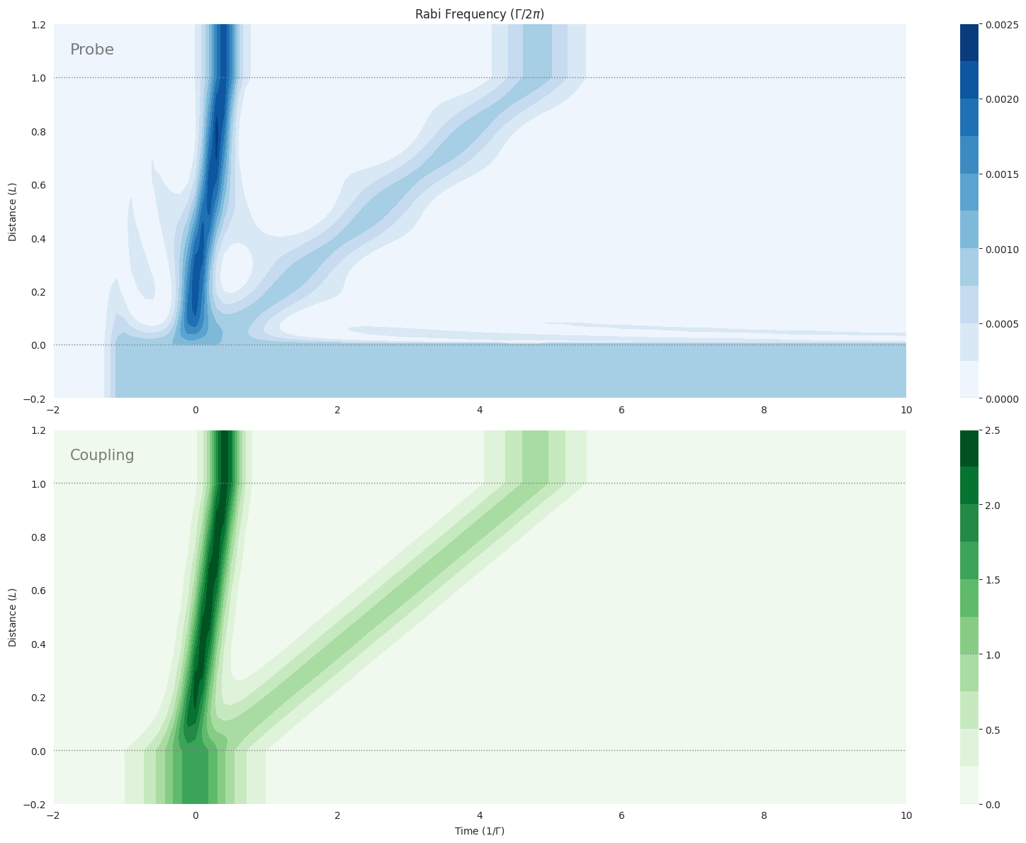
Double optical surfer — 4π coupling soliton on CW probe
As for the 2π optical surfer, but with a 4π coupling soliton (\(\theta_\mathrm{coupling} = 4\pi = 2 \times 2\pi\)). The higher area produces two surfer solitons: the coupling pulse generates a pair of probe brightening regions that both propagate through the medium.
[20]:
ampl_surf4 = 4.0 / t_width / (2 * np.pi)

mb_solve_json_surf4 = """
{
  "atom": {
    "fields": [
      {
        "coupled_levels": [[0, 1]],
        "detuning": 0.0,
        "detuning_positive": true,
        "label": "probe",
        "rabi_freq": 1.0e-3,
        "rabi_freq_t_args": {"ampl": 1.0, "on": -1.0, "fwhm": 0.3796628587572578},
        "rabi_freq_t_func": "ramp_on"
      },
      {
        "coupled_levels": [[0, 2]],
        "detuning": 0.0,
        "detuning_positive": true,
        "label": "coupling",
        "rabi_freq": 1.6768028730843334,
        "rabi_freq_t_args": {"ampl": 1.0, "centre": 0.0, "width": 0.3796628587572578},
        "rabi_freq_t_func": "sech"
      }
    ],
    "num_states": 3
  },
  "t_min": -2.0,
  "t_max": 10.0,
  "t_steps": 120,
  "z_min": -0.2,
  "z_max": 1.2,
  "z_steps": 140,
  "z_steps_inner": 2,
  "interaction_strengths": [10.0, 10.0],
  "savefile": "mbs-vee-weak-cw-sech-4pi"
}
"""

mbs_surf4 = mb_solve.MBSolve().from_json_str(mb_solve_json_surf4)
mbs_surf4.mbsolve(recalc=False);
[21]:
fig = plt.figure(figsize=(16, 12))

ax = fig.add_subplot(211)
cf = ax.contourf(mbs_surf4.tlist, mbs_surf4.zlist,
                 np.abs(mbs_surf4.Omegas_zt[0] / (2 * np.pi)),
                 np.linspace(0.0, 2.5e-3, 11), cmap=plt.cm.Blues)
ax.set_title(r"Rabi Frequency ($\Gamma / 2\pi$)")
ax.set_ylabel("Distance ($L$)")
ax.text(0.02, 0.95, "Probe", va="top", ha="left", transform=ax.transAxes,
        color="k", fontsize=16, alpha=0.5)
plt.colorbar(cf)

ax = fig.add_subplot(212)
cf = ax.contourf(mbs_surf4.tlist, mbs_surf4.zlist,
                 np.abs(mbs_surf4.Omegas_zt[1] / (2 * np.pi)),
                 np.linspace(0.0, 2.5, 11), cmap=plt.cm.Greens)
ax.set_xlabel(r"Time ($1/\Gamma$)")
ax.set_ylabel("Distance ($L$)")
ax.text(0.02, 0.95, "Coupling", va="top", ha="left", transform=ax.transAxes,
        color="k", fontsize=15, alpha=0.5)
plt.colorbar(cf)

for ax in fig.axes:
    for y in [0.0, 1.0]:
        ax.axhline(y, c="grey", lw=1.0, ls="dotted")
plt.tight_layout()
[22]:
total_area = np.sqrt(mbs_surf4.fields_area()[0]**2 + mbs_surf4.fields_area()[1]**2)

fig, ax = plt.subplots(figsize=(16, 4))
ax.plot(mbs_surf4.zlist, mbs_surf4.fields_area()[0] / np.pi, label="Probe", clip_on=False)
ax.plot(mbs_surf4.zlist, mbs_surf4.fields_area()[1] / np.pi, label="Coupling", clip_on=False)
ax.plot(mbs_surf4.zlist, total_area / np.pi, label="Total", ls="dashed", clip_on=False)
ax.legend()
ax.set_ylim([0.0, 4.0])
ax.set_xlabel("Distance ($L$)")
ax.set_ylabel(r"Pulse Area ($\pi$)");